Game Theory and Real Options:
Analysis of Land Value and Strategic Decisions
in Real Estate Development
by
Chun Kit So ( Timothy So )
Bachelor of Science in Architecture, University of Virginia, 2003 Submitted to the Program in Real Estate Development in Conjunction with the Center for Real Estate In Partial Fulfillment of the Requirements for the Degree of
Master of Science in Real Estate Development at the
Massachusetts Institute of Technology September, 2013
©2013 Chun Kit So All rights reserved
The author hereby grants to MIT permission to reproduce and to distribute publicly paper and electronic copies of this thesis document in whole or in part in any medium now known or hereafter created.
Signature of Author______________________________________________________________ Center for Real Estate July 30, 2013 Certified by____________________________________________________________________ Walter Torous Senior Lecturer, Center for Real Estate
Thesis Supervisor Accepted by___________________________________________________________________ David Geltner Chair, MSRED Committee, Interdepartmental Degree Program in Real Estate Development
Game Theory and Real Options:
Analysis of Land Value and Strategic Decisions
in Real Estate Development
by
Chun Kit So ( Timothy So )
Submitted to the Program in Real Estate Development in Conjunction with the Center for Real Estate on July 30, 2013
In Partial Fulfillment of the Requirements for the Degree of Master of Science in Real Estate Development
ABSTRACT
This thesis investigates the use of the game theory and the real options theory in real estate development at the strategic level, trying empirically to explain different economic observations among different metropolitan cities and different property types.
The real options theory provides a rich theoretical framework to analyze investment values in real estate development. It takes the market uncertainty into consideration, while the widely used neoclassical NPV valuation method takes a deterministic approach. A simplified real options valuation model is set up in this thesis to calculate the option premium value of waiting for developers. However, since it is done in a monopolistic setting, the strategic interaction aspect of real estate development will be analyzed using the game theory model. The interaction of the game theory model and the real options model will provide a comprehensive and powerful framework to study the timing strategy of developers.
Using data spanning quarterly from 1995 to 2013 among 5 property types (single-family house, apartment, industrial, office, and retail) and 44 MSAs, this thesis analyzes the relationships empirically between the volatility of underlying assets, the land cost ratio, the option premium value, and the timing of development. The aims of the study are twofold. First, the study compares different market characteristics among different MSAs and different property types from the option game theoretic perspective. Second, it analyzes the effect and the use of the game theory and the real options theory in the context of real estate development.
ACKNOWLEDGEMENT
I would like to sincerely thank Professor Walter Torous for his guidance, insight, and dedication as the supervisor of this thesis. From the very beginning, his comments and advices inspired me a lot, and his vast experience always helped me move forward. I am also grateful that he allows me to have enough flexibility to pursue a topic that I am most interested in and I truly learn a lot in the process.
I am also very thankful to Professor David Geltner, who always patiently answers all my real estate finance questions in detail; Professor Bill Wheaton, who guides me to narrow down my topic and provides me with the data that I need; Professor Robert Merton, who helps me tremendously on the concepts of options pricing; Professor Stewart Myers, who inspires me to look at real options from a different perspective; Professor Alessandro Bonatti, who guides me diligently on the strategic concepts of game theory; and Professor Steven Grenadier, who provides me with suggestions and resources on the topics of game theory. I would also like to thank RCA, CBRE, R.S. Means, and Lincoln Institute of Land Policy for providing me with the valuable data for the analyses in this thesis.
I would also like to thank all my fellow classmates, the faculty, and the staff at CRE for making this year at MIT such a fabulous experience.
Last but not least, I am very grateful to have my wife, Joyce So, and my parents, Pauline and Danny So, who always give me unconditional love and support in so many ways this year, and in all of my endeavors. Without them, my study at MIT this year would not be possible. I am also thankful to have my children, Lyla and Karlan, for being around to give me the distractions that I need most during challenging times.
Thank you. Timothy So July, 2013
LIST OF TABLES
Table 2.0: Game Payoff Matrix Example………...………..…………. 23
Table 2.1: Game Theory Model Setup……….………...………..…………. 24
Table 2.2a: Scenario 1: Develop-Develop Equilibrium………..………..…………. 27
Table 2.2b: Scenario 2: Develop-Develop / Wait-Wait Equilibrium…………...…………. 27
Table 2.2c: Scenario 3: Develop-Wait / Wait-Develop Equilibrium…………...…………. 28
Table 2.2d: Scenario 4: Wait-Wait Equilibrium………...………..………..…………. 28
Table 2.3: Numerical Example Game Payoff Matrix Result………...…….…………. 31
Table 4.0: 30 Metropolitan Statistical Areas for Commercial Markets Analysis…….……. 40
Table 4.1: Volatility and Land Cost Ratio Regression Results for Commercial Markets…. 42 Table 4.2: Volatility and Land Cost Ratio Summary for Commercial Markets……...……. 43
Table 4.3: 44 Metropolitan Statistical Areas for Residential Markets Analysis……...……. 45
Table 4.4: Volatility and Land Cost Ratio Summary for Residential Markets……….……. 47
Table 4.5: Volatility Analysis Summary for Commercial and Residential Markets………. 48
Table 4.6: Land Cost Ratio Analysis Summary for Commercial and Residential Markets.. 48
Table 5.0: Time-Series Analysis Regression Results for Commercial Markets……...……. 52
Table 5.1: Time-Series Analysis Area-Adjusted Regression Results………..…....….……. 54
Table 5.2: Time-Series Analysis Summary……….…....….……. 54
Table 5.3: Cross-Sectional Analysis Regression Results for Commercial Markets….……. 55
Table 5.4: Cross-Sectional Analysis Area-Adjusted Regression Results….………. 56
Table 5.5: Cross-Sectional Analysis Summary………..……….…....….……. 57
Table 5.6: Time-Series Analysis Regression Results for Residential Markets………. 58
Table 5.7: Time-Series Analysis Area-Adjusted Regression Results………..…....….……. 58
Table 5.8: Cross-Sectional Analysis Regression Results for Residential Markets….…..…. 59
Table 5.9: Cross-Sectional Analysis Area-Adjusted Regression Results…………...…..…. 60
Table 5.10: Symmetric Game Theory Model Setup…...……….…....….……. 62
Table 5.11: Office Game Payoff Matrix………...……….…....….……. 64
Table 5.12: Retail Game Payoff Matrix…….………...……….…....….……. 64
Table 5.13: New York Office Game Payoff Matrix…….………...………..…....….……. 65
Table 5.14: Dallas Office Game Payoff Matrix…….………...…………...…....….……. 66
Table 5.15: San Francisco Single-Family House Game Payoff Matrix…….………...……. 67
Table 5.16: Boston Single-Family House Game Payoff Matrix…………....………...……. 67
Table 5.17: Washington DC Single-Family House Game Payoff Matrix……….…...……. 67
Table 5.18: Phoenix Single-Family House Game Payoff Matrix……….….…...……. 67
Table 5.19: New Orleans Single-Family House Game Payoff Matrix…….…….…...……. 68
Table 5.20: Atlanta Single-Family House Game Payoff Matrix………...…...……. 68
LIST OF FIGURES
Figure 2.0: Real Options Binomial Tree Diagram………. 17 Figure 2.1: Numerical Example Binomial Tree Result………. 18 Figure 2.2: Optimal Actions Binomial Tree Result………..…………. 19
TABLE OF CONTENTS Abstract……….. 2 Acknowledgement………. 3 List of Tables………. 4 List of Figures………...………. 5 1.0 Chapter 1: Introduction……….. 8
1.1 Purpose of the thesis……….………... 8
1.2 Research motivation & hypothesis……….………. 9
1.3 Research methodology……….……… 10
1.4 Results & interpretation………... 12
2.0 Chapter 2: Overview of Fundamentals……….. 14
2.1 Real Options………. 14
2.1.1 Real Options Pricing Model setup………. 15
2.1.2 Strategic implication of real options pricing model………... 20
2.2 Game Theory………...…… 23
2.2.1 Payoff Matrix Setup for Real Estate Development……… 24
2.2.2 Strategic implication of the Real Estate Development Game Theory Payoff Matrix……….. 27
3.0 Chapter 3: Literature review……….. 33
3.1 Real Options in Real Estate Development………. 33
3.2 Empirical Testing of Real Options in Real Estate Development…………... 34
3.3 Game Theory in Real Estate Development……… 35
3.4 Land Value Studies……… 38
4.0 Chapter 4: Methodology & Data Collection……….. 39
4.1 Commercial Real Estate Asset and Land Value Data……….. 39
4.1.1 Use of Real Capital Analytics (RCA) data……...………. 39
4.1.2 Comparison between 30 Metropolitan Statistical Areas (MSAs)..… 40
4.2 Residential Real Estate Asset and Land Value Data………... 44
4.2.1 Use of the Lincoln Institute of Land Policy data……..………. 44
4.2.2 Comparison between 44 Metropolitan US cities….………..……… 45
4.3 Data Summary………. 47
4.4 Strengths & weaknesses of methodology……… 49
5.0 Chapter 5: Data analysis & Interpretation………... 50
5.1 Empirical Testing of the Real Options Pricing Model……..……….. 50
5.1.1 Regression results - Commercial Real Estate……… 52
(1) Across Time within a MSA………..… 52
(2) Across MSAs within a Time period……….… 55
5.1.2 Regression results - Residential Real Estate………..……… 58
(1) Across Time within a MSA………..… 58
(2) Across MSAs within a Time period……….… 59
5.1.3 Summary of the results……….. 60
5.2 Application of Game Theory Payoff Matrix……….... 62
5.2.1 Strategic Implication in Commercial Real Estate……….. 63
5.2.2 Strategic Implication in Residential Real Estate……….………... 67
5.2.3 Summary of the results………..……… 69
5.3 Evaluation of the use of Game Theory and Real Options in Real Estate Development……….……….. 71
5.3.1 Benefits and Advisory Power of the method………. 73
(1) Real Options Model……….…… 73
(2) Game Theory Model………..……….. 74
(3) Regression Analysis from Option Game Theoretic Perspective.. 74
5.3.2 Limitation of the method………... 75
(1) Real Options Model……….…… 75
(2) Game Theory Model………..……….. 76
6.0 Chapter 6: Conclusions………... 77
6.1 Conclusion………... 77
6.2 Topics for further study………... 81
1.0 Chapter 1: Introduction
1.1 Purpose of the thesisThis thesis investigates the use of game theory and real options in real estate development at a strategic level, backed up by empirical data to try to explain different economic observations among different regions and metropolitan cities.
The real options approach to analyzing investment under uncertainty has become part of the mainstream literature of financial economics. Essentially, the real options approach to analyze the opportunity to invest in a project is analogous to an American call option on the investment opportunity. Once that analogy is made, the vast and rigorous machinery of financial options theory can be applied to analyze such investment option. The real options approach is well summarized in Dixit and Pindyck (1994) and Trigeorgis (1996). The most well-known result of the real options literature is the invalidation of the
standard net present value (NPV) rule of investing in any project with a non-negative net present value. The optimal investment rule, as described in the real options literature, is to invest when the asset value exceeds the investment cost by a potentially large option premium. While the widely used neoclassical NPV valuation method takes a
deterministic approach, the real options valuation method takes into account the option value created by uncertain future outcome.
Since the 1980s, there have been lots of interest in academic research in real options valuation methods. A vast array of models and frameworks have been studied and proposed. Titman (1985), Williams (1991), and Trigeorgis (1996) provide some of the most influential conceptual frameworks in the field, especially as applied to real estate development. While the real options valuation gives a more comprehensive picture of investment value as compared to the neoclassical NPV valuation method, it is done in a monopolistic setting. That is partially the reason why the real options valuation is not applied in real-world situations as often as it should be because economic markets are
The option value as described in real options pricing methods is not an accurate
representation of project value as valuated by firms. Grenadier (1996), and Schwartz and Torous (2007) demonstrate that competitions among real estate developers erodes the option value, and illustrate that the real options valuation method alone is not
comprehensive enough to reflect real-world situations. Strategic interactions are essential components to be considered in the valuation process. Therefore, the application of the game theory in the real options analysis will provide important insights at a strategic level. And this thesis empirically compares the implication of the game theory and the real options in real estate development among 4 regions (East, Midwest, South, and West), 44 metropolitan cities, and 4 property types (Apartment, Industrial, Office, and Retail) for commercial markets, and single-family houses for residential markets.
1.2 Research motivation & hypothesis
Real estate development is one of the classic applications of the real options. As in Titman (1985) and Williams (1991), the development of real estate is analogous to an American call option on a building, where the exercise price is equal to the construction cost. An option is a contract or situation that gives its holder the right but not the
obligation to buy (if a call) or sell (if a put) a specified asset (e.g. common stock or project) by paying a specified cost (the exercise or strike price) on or before a specified date (the expiration or maturity date). If the option can be exercised before the maturity, it is an American option; if only at the maturity, a European option. In real estate
development, if the value of a building is higher than the cost of construction, the residual value is what developers can pay for the land to make it a zero NPV project. In other words, the land value is analogous to the option value. By holding on to the piece of land and deferring development, the intrinsic value of the land would be higher than the residual value as demonstrated in Quigg (1993). Some numerical examples will be illustrated in following chapters. Taken literally, the standard, myopic real options approach implies that developers should ignore the construction behavior of their competitors. However, in real estate markets, developers are likely to face considerable competitions from competitors, and the development activities of competitors will have a
fundamental impact on one’s development options. By extending the options framework to account for strategic interaction, a much richer set of investment implications is obtained. While the standard real options models dictate that a developer should wait until the development option is considerably in-the-money, which means that the value of a building is much larger than the cost of construction, competitions and the fear of pre-emption will likely force developers to build much earlier. In addition, while standard real options models imply that developments will be simultaneous, game-theoretic models allow for the possibility of sequential developments. Competitive models of real estate development can also help explain boom-and-bust behavior in commercial
constructions, as well as why rational developers may construct new buildings in the face of declining demand and market values as illustrated in Grenadier (1996).
Regarding the interaction of the real options and the game theory, the timing strategy of real estate developers has long been a complex issue to study, affected by many external economics forces. This thesis focuses on the relationships of the land value, the land cost ratio, and the volatility of underlying assets in different regions and metropolitan cities, trying to explain developers’ timing strategy in different markets depending on those variables from an option game theoretic perspective. Intuitively, when the volatility of underlying assets is high and the land cost ratio is high, the timing option value will be high too, which implies that developers should wait to observe the market trend better before exercising the option to develop or redevelop the piece of land. A large set of data spanning from as early as 1995 to 2013 across 4 regions, 44 metropolitan cities, and 4 property types will be used to analyze the relationship and discrepancy between the observed data and results predicted by the option game theoretic approach.
1.3 Research methodology
Asset values of 4 property types (Apartment, Industrial, Office, and Retail) in 30 Metropolitan Statistical Areas (MSA) spanning from 2001 to 2013 are collected from Real Capital Analytics, Inc (RCA) for the commercial portion of the study. Construction
values of single-family houses in 44 MSAs spanning from 1995 to 2013 are collected from Lincoln Institute of Land Policy for the residential portion of the study. For the commercial portion, the construction activity is measured by number of square feet completed (industrial, office, and retail) and number of units completed (apartment), with data collected from CBRE. For the residential portion, the construction activity is
measured by number of permits issued for single-family houses, with data collected from U.S. Census Bureau.
Using the real options pricing model described in detail in section 2.1.1, the option premium, defined as the difference between the option value of waiting and the residual land value, is calculated for each property use in each MSA within a certain given time period. The option premium is a value indicating theoretically the magnitude of benefits for a developer to wait, rather than to develop now. This is a better indicator than the absolute option value of waiting because the option premium eliminates the distorted effect of different asset value ranges for different uses in different MSAs. For example, given everything the same, higher asset values by definition will always give higher option values because the subject in question is of higher values, which will falsely imply that office developers will always have a higher benefit of waiting compared to industrial developers because of their inherently higher absolute option values of waiting. When compared across different uses and MSAs, the option premium should be used to measure the magnitude of incentive for developers to wait.
To study the relationship between the option premium, the land cost ratio, and the timing strategy of developers, the following regression is applied to measure the degree of correlation:
CA = α + β (Cp) + γ (LCR) + ɛ
Where CA = Construction Activity
Cp = Option Premium value
= Ct - (St - Kt )
LCR = Land Cost Ratio = !!!!
S = property asset value
K = construction / replacement cost
In this thesis, two levels of relationships are studied: (1) across time within a MSA, and (2) across MSAs within a time period for both the commercial and residential markets. Sections 4.0 and 5.0 will further elaborate all the details.
1.4 Results & interpretation
As presented in detail in sections 4.0 and 5.0, for commercial markets, the higher the asset value volatility is, the higher the option premium value will be, and the lower the level of construction activities will result. Meanwhile, the higher the land cost ratio is, the lower the level of construction activities will result. At an aggregate level across multiple MSAs, apartment developments are the most sensitive to the option premium value, followed by industrial and office developments. Retail developments are the least sensitive to the option premium value. Compared between the time-series (across time within a MSA) study and the cross-sectional (across multiple MSAs within a time period) study, the time-series study seems to show higher sensitivity to the option premium value than the cross-sectional study does. The time-series study also shows more significant regression results than the cross-sectional study does (sections 4.1 and 5.1.1).
For residential markets, results between the time-series study and the cross-sectional study are not as consistent as those of the commercial markets study. In the time-series
and the lower the level of construction activities will result. Meanwhile, the lower the land cost ratio is, the lower the level of construction activities will result. However, the cross-sectional study shows the opposite. Compared between the time-series study and the cross-sectional study, the time-series study again seems to show higher sensitivity to the option premium value than the cross-sectional study does. Between commercial markets and residential markets, the regression results show that residential markets are more sensitive to the option premium value than commercial markets do. Residential markets also show more significant regression results than commercial markets do (sections 4.2 and 5.1.2). Overall, the correlation is a lot stronger between the option premium value and the level of construction activity than that between the land cost ratio and the level of construction activity. In the Variance Inflation Factor tests for the issue of multi-collinearity, both results of commercial markets and residential markets show that the correlation between the option premium value and the land cost ratio is not strong or problematic enough to distort their effect on the level of construction activity (section 5.3).
2.0 Chapter 2: Overview of Fundamentals
2.1 Real OptionsThe real options valuation, also often termed the real options analysis (ROV or ROA), applies option valuation techniques to capital budgeting decisions. A real option itself is the right, but not the obligation, to undertake certain business initiatives, such as
deferring, abandoning, expanding, staging, or contracting a capital investment project. Dixit and Pindyck (1994) have explained investment decisions in detail in their book. They site that most investment decisions share three important characteristics. First, the investment is partially or completely irreversible. Second, there is uncertainty over the future rewards from the investment. Third, some flexibility about the timing of the investment usually exists. These three characteristics interact to determine the optimal decisions for any investor.
Within the neoclassical theory of investment, the net present value (NPV) theory, has not recognized the interaction between irreversibility, uncertainty, and the choice of timing. Real world investments seem less sensitive to changes in the interest rate and the tax policy, and much more sensitive to the volatility and the uncertainty over the economic environment. A growing body of literature has shown that the ability to delay an irreversible investment can profoundly affect the decision to invest. The traditional Discounted Cash Flow (DCF) method dictates that companies should not execute any negative NPV project. The new view of investment opportunities as options has shown that the traditional NPV rule can give very wrong answers unless all relevant option values are included in the NPV. Note that if choices are investing now or never, the standard NPV rule applies because there is no option to wait years.
2.1.1 Real Options Pricing Model setup
When applied in real estate development, the real options can be considered an American call option on the asset value of a building with the exercise price being the construction or replacement cost. When the construction or replacement cost is subtracted from the asset value of the building, the residual value is the maximum price that a developer should pay for the piece of land to make it a zero NPV project. As stated above, this classic NPV approach neglects the option value of waiting for future development. If the real options pricing model is applied in the decision-making process, the option value should be considered as well. In each period, developers should compare the residual value with the option value to better understand their optimal action. The option premium value (Cp) is defined as the difference between the residual value and the option value. If
the option premium value is positive, it means that the option value is higher than the residual value, and the option to wait is more valuable than the decision to develop the piece of land in this period, vice versa. A fundamental and pure form of the real options pricing model will be used in this thesis to examine empirically the relationship between the land value and the timing strategy of developers. Time t=0 is defined as the initial period when the decision is about to be made. The property asset value (St) will either go
up by a multiple (u) to (St+0.25 = uSt) with the probability (p) or go down by a multiple (d)
to (St+0.25 = dSt) with the probability (1-p). The construction or replacement cost will
increase at an average growth rate throughout the periods. Since it is an American call option, the option value (Ct) is defined as the maximum value between the residual value
St = e-rt [ p x uSt + (1-p) x dSt ] Kt = e-gt Kt+0.25 Ct = max { St - Kt , e-rt [ p x Cu t+0.25 + (1-p) x Cd t+0.25] } Cp = Ct - (St - Kt ) p = !!!!"!!! u = 𝑒! ! d = 𝑒!! !
Where: S = property asset value per sq.ft.
K = construction / replacement cost per sq.ft.
C = option value of waiting
Cp = option premium value
p = probability of value moving upward
u = multiple of value moving upward
d = multiple of value moving downward
σ = volatility of value
r = risk-free rate
g = construction cost growth rate
Volatility of value or cost is calculated using historical data with the following equations:
ΔS = ln(! !!
!!!.!")
SD = (!!!)!!! !
t = 0 t = 0.25 t = 0.5 t = 0.75 t = 1 uuuuS uuuS uuS uuudS p uS uudS S udS uuddS 1-p dS uddS ddS udddS dddS ddddS K K0.25 K0.5 K0.75 K1 Cuuuu Cuuu Cuu Cuuud p Cu Cuud C Cud Cuudd 1-p Cd Cudd Cdd Cuddd Cddd Cdddd
A numerical example is illustrated as follows. In a given city, the volatility of asset value of office buildings is 20% and the growth rate of construction or replacement cost is 5%. At t=0, the asset value of office building is $100 per sq.ft. while the construction cost is $70 per sq.ft. The Risk-free rate is assumed to be 5%. Using equations presented above, the real options binomial tree is as follows:
t = 0 t = 0.25 t = 0.5 t = 0.75 t = 1 149.18 73.59 134.99 75.59 72.67 122.14 62.31 122.14 71.77 73.59 110.52 50.37 110.52 48.55 70.88 72.67 S=100 39.64 100 37.84 100 K=70 71.77 73.59 C=30.28 90.48 28.23 90.48 26.41 70.88 72.67 20.23 81.87 17.81 81.87 71.77 73.59 11.47 74.08 8.28 72.67 4.40 67.03 73.59 0
Figure 2.1: Numerical Example Binomial Tree Result
In this example, the residual land value is $30 per sq.ft. while the option value of waiting is $30.28 per sq.ft. The option premium value (Cp) is $0.28 per sq.ft. This implies that
office developers in this city should rationally wait to develop, rather than to exercise the option to develop at t=0. In theory, if the real options pricing model is applied to evaluate the land value, office developers in that city should be logically willing to pay up to $30.28 per sq.ft. on average for a piece of land to account for the option value. In fact, Quigg, L. (1993) examines the empirical predictions of a real options pricing model using
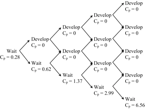
incorporates the option to wait to develop land. The option model has explanatory power for predicting transactions prices over and above the residual value. Market prices reflect a premium for the option to wait to invest that has a mean value of 6% in their samples. Option values shown in bold and underlined indicate nodes where early exercise is optimal. In other words, in those nodes, the option premium value is compressed to a point which equals the residual land value. Therefore, developers have no incentive to wait but to exercise the option to develop, as illustrated in the binomial tree below:
Develop Cp = 0 Develop Cp = 0 Develop Develop Cp = 0 Cp = 0 Develop Develop Cp = 0 Cp = 0
Wait Develop Develop
Cp = 0.28 Cp = 0 Cp = 0 Wait Develop Cp = 0.62 Cp = 0 Wait Develop Cp = 1.37 Cp = 0 Wait Cp = 2.99 Wait Cp = 6.56
2.1.2 Strategic implication of the real options pricing model
As illustrated with the model in Section 2.1.1, when the residual land value is less than the option value of waiting, developers should wait to develop. Based on the model, the magnitude of the option premium (Cp) is affected by the following variables: (1) the
volatility of asset value, σs, (2) the growth rate of construction or replacement cost, g, (3)
the maturity date of option, T, and (4) the risk-free rate, r.
(1) Volatility of asset value, σs
The option premium is an increasing function of the volatility of asset value:
!!! !!! > 0
As the volatility of asset value increases, the option premium value will increase as well. That makes intuitive sense because the option of waiting becomes more
valuable if the future asset value is more uncertain. In cities with a higher volatility of asset values, more developers are expected to wait before they decide to exercise the option when asset values are more favorable to them.
(2) Growth rate of construction or replacement cost, g
The option premium is a decreasing function of the growth rate of the construction or replacement cost:
!!!
!! < 0
As the growth rate of the construction or replacement cost increases, the option premium value will decrease. Intuitively, when the construction cost escalates faster,
option value of waiting is diminished if the growth rate of the construction cost is high. Therefore, in cities where the construction or replacement cost increases faster, more developers are expected to exercise the development option earlier.
(3) Maturity date of option, T
The option premium is an increasing function of the maturity date of option, T:
!!! !" > 0
As the duration of option-exercising periods increases, the option premium value will increase. Conceptually, if external factors in the market allow developers to wait longer, the option premium will be higher, all things being equal. The Maturity date of the real options in real estate development can be considered a time by which developers lose the flexibility of choosing between developing immediately and waiting to develop. That maturity date depends on external factors in the market such as the level of competitions, land policy revisions, and a shift in market demand and internal factors of the developer such as the corporate investment time frame, the development schedule, and various business strategies. Grenadier, S. R., and Wang, N. (2006) interestingly show that developers are very impatient about choices in the short-term, but are quite patient when choosing between long-term alternatives. That paper indirectly demonstrates that when the maturity date of the option is further away from now, the option premium value will be higher and thus developers tend to keep the option of waiting more. It is noted that in this study, the maturity date of option is kept the same for comparison purposes across different cities and property types.
(4) Risk-free rate, r
The option premium is an increasing function of the risk-free rate, r:
!!! !" > 0
As the risk-free rate increases, the option premium value will increase. Intuitively, when the risk-free rate increases, the opportunity cost of investment will increase too. That makes the option value of waiting higher, vice versa. Therefore, when the risk-free rate is low, more developers will tend to exercise their option to develop earlier. It is noted that this model assumes a constant risk-free rate for comparison purposes across different cities and property types.
As the volatility of asset value and the growth rate of the construction or replacement cost are different among different cities and different property types, the timing behavior of developers are influenced by different option premium values under different situations. This thesis will examine if developers behave according to results predicted by the real options pricing model presented in previous sections. Then, the game theory presented in coming sections will be applied to understand further any discrepancy found in our empirical study.
2.2 Game Theory
The game theory is the study of strategic decision-making. It is a discipline that studies situations of strategic interaction. In many real-world situations, the action of one player affects the pay-off of other players. The application of the game theory provides a strategic framework to analyze the best response of each player’s action. In the game theory, a solution concept is a formal rule predicting which strategies will be adopted by players, therefore predicting the result of the game. A strategy consists of a rule
specifying which actions a player should take given the actions taken by other players. The most commonly used solution concepts are equilibrium concepts. An equilibrium is a configuration of strategies where each player’s strategy is his best response to the
strategies of all the other players. The principle concept is illustrated in the following simplified example.
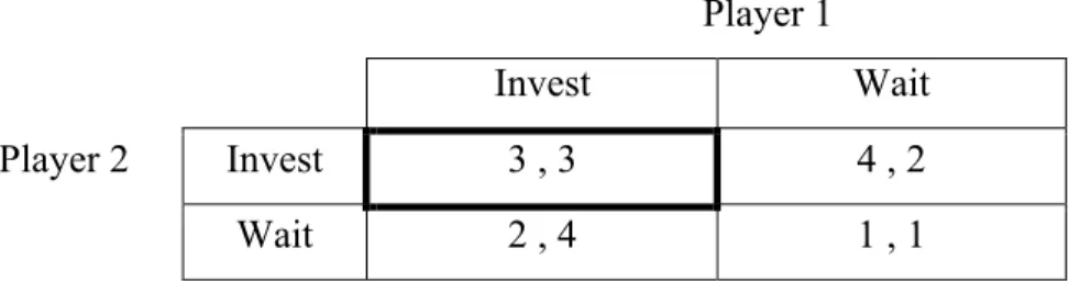
In an efficient market, assuming it is a symmetric game, both rational player 1 and player 2 have the option to invest now or to wait to invest in next period. The pay-off matrix of player 1 and player 2 is shown in Table 2.0, with pay-offs on the left referring to those of player 2 while pay-offs on the right referring to those of player 1.
Player 1
Player 2
Invest Wait
Invest 3 , 3 4 , 2
Wait 2 , 4 1 , 1
Table 2.0: Game Payoff Matrix Example
The game pay-off matrix describes four possible outcomes. If both players invest, each of them gets a off equal to 3. If player 1 invests while player 2 waits, they will get pay-offs of 4 and 2 respectively. If both players wait, they will each get a pay-off of 1. In this symmetric game, when player 1 invests, the best response of player 2 is to invest as well to maximize its pay-off. When player 1 waits, the best response of player 2 is to invest
because the pay-off of investing now is bigger than that of waiting. Applying this logic to all possible scenarios, there is an equilibrium, as indicated with a bold box, in this game, which is that both players should invest now. In this simplified symmetric game, the application of game theoretical principles shows that the best response for both players is to invest now because that is the equilibrium of this game. A few other examples in later sections will show that there may be multiple equilibria in other games and discuss its implications.
2.2.1 Payoff Matrix Setup for Real Estate Development
In real estate development, the real-world situation is usually too complex for one model to analyze the optimal development strategy accurately. However, the interaction of the real option valuation and the game theory can provide a strategic framework to help better understand the interactive investment opportunity and to offer important strategic implications. The following model will be used to analyze the empirical data presented in this thesis.
In this simplified setting, two developers have the option to develop now or to wait to develop in next period. If a developer develops, its pay-off is defined as the property asset value minus the construction or replacement cost. If a developer waits, its pay-off is defined as the option value of waiting. See Table 2.1 for the pay-off matrix of these two developers. Developer 1 Developer 2 Develop Wait Develop ωD2 St – Kte-rt , ωD1 St – Kte-rt ωL2 St – Kte-rt , Ct1fw Wait Ct2fw , ωL1 St – Kte-rt Ct2 , Ct1
Where: St = property asset value per sq.ft. at time = t
Kt = construction / replacement cost per sq.ft. at time = t
ωD1 = proportion of value for developer 1 when both developers
develop
ωD2 = proportion of value for developer 2 when both developers
develop
ωL1 = proportion of value for developer 1 when developer 1
develops first (Leader)
ωL2 = proportion of value for developer 2 when developer 2
develops first (Leader)
ωF1 = proportion of value for developer 1 when developer 1
waits (Follower)
ωF2 = proportion of value for developer 2 when developer 2
waits (Follower)
Ct1 = option value of waiting for developer 1 when both developers
wait (no Leader)
Ct2 = option value of waiting for developer 2 when both developers
wait (no Leader)
Ct1fw = option value of waiting for developer 1 when developer 1 waits
(Follower)
= max (ωF1 St+1 – Kt+1e-r(t+1) , e-r(t+1) [q Cu(t+1)1fw + (1-q) Cd(t+1)1fw ] )
Ct2fw = option value of waiting for developer 2 when developer 2 waits
(Follower)
= max (ωF2 St+1 – Kt+1e-r(t+1) , e-r(t+1) [q Cu(t+1)2fw + (1-q) Cd(t+1)2fw ] )
The pay-off matrix is designed to capture a few important elements in the strategic planning process of real estate development. At a conceptual level, the simplified model reflects factors including the nature of developers, the nature of market, and the nature of timing.
Firstly, for example, if two office developers are players of the game, when they decide to develop at the same time, their pay-offs will depend on their strength to capture the market demand, which will be reflected by ωD1 and ωD2 (where ωD1 < ωD2 < 1 if developer
2 is a stronger player). When two complementary developers, such as office and retail developers, are players of the game, the pie will actually grow bigger when they develop at the same time, reflected by ωD1 and ωD2 (where ωD1 ≤≥ωD2 > 1). Therefore, the nature
of developers would affect their pay-offs, which affects their optimal strategies accordingly.
Secondly, market conditions affect how developers react to the market demand. For example, if the demand for residential space in certain submarkets is finite and known, developing alone will always yield a higher pay-off than competing with other developers to split the market, as indicated by ωD1 and ωL1 (where ωD1 < ωL1). In a different scenario,
if the demand for retail space will increase through collaboration, retail developers will both get a higher pay-off when they develop together, as indicated by ωD1 and ωL1 (where
ωD1 > ωL1). Therefore, the nature of market has strategic implications for actions of
developers from a game theoretic perspective.
Thirdly, like in other types of investments, the timing is essential to successful
development projects. It is instrumental in determining the pay-offs in interactive games. For example, if the demand for more office space is obvious and the volatility of office building value is low, developers have less incentive to wait, i.e. they would rather be a Leader than a Follower to capture the First Mover Advantage (FMA) as reflected by ωL1
and ωF1 (where ωL1 > ωF1). However, if the demand is uncertain and the new market
requires synergy to enhance new demand, developers have more incentive to wait, i.e. they would rather be a Follower than a Leader to capture the Second Mover Advantage (SMA) as reflected by ωL1 and ωF1 (where ωL1 < ωF1). Therefore, the nature of timing
affects interactive decisions of developers. As illustrated above, these three important factors are indicated by variables ωDi, ωLi, and ωFi in the model. In the next section, their
a numerical example will be used at the end of the section to tie the real options valuation model and the game theory model together to make the framework clearer.
2.2.2 Strategic implication of the Real Estate Development Game Theory Payoff Matrix
From a game theoretic perspective, the action of Developer 1 and that of Developer 2 are mutually affected by each other. If both developers are rational players, they should all choose the equilibrium action to maximize their pay-offs. Once in equilibrium, no one can improve its pay-off by switching its decision. In the context of real estate
development, the real option is irreversible. That is, once a developer decides to “develop”, it cannot switch back to the “wait” option. Therefore, developers are
sometimes stuck in the sub-optimal situation. Based on the simplified model presented in the previous section, there are four equilibrium or multi-equilibria scenarios in a
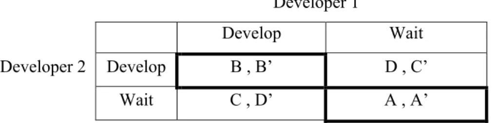
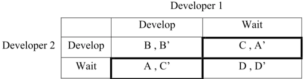
symmetric game with different variations in an asymmetric game. See Tables 2.2a to 2.2d for the four scenarios.
Developer 1
Developer 2
Develop Wait
Develop C , C’ A , D’
Wait D , A’ B , B’
Table 2.2a: Scenario 1: Develop-Develop Equilibrium
Developer 1
Developer 2
Develop Wait
Develop B , B’ D , C’
Wait C , D’ A , A’
Developer 1
Developer 2
Develop Wait
Develop B , B’ C , A’
Wait A , C’ D , D’
Table 2.2c: Scenario 3: Develop-Wait / Wait-Develop Equilibrium
Developer 1
Developer 2
Develop Wait
Develop D , D’ B , C’
Wait C , B’ A , A’
Table 2.2d: Scenario 4: Wait-Wait Equilibrium
Where: Value of A > B > C > D and Value of A’ > B’ > C’ > D’ and
Whether A > A’ or B > B’ or C > C’ or D > D’ depends on relative value of ωD1 & ωD2, ωL1 & ωL2, and ωF1 & ωF2.
As explained in section 2.2, the equilibrium state in this model can be determined by comparing the pay-offs of each player given the action taken by another player. For example, in scenario 1, if Developer 1 decides to “develop”, the best response of Developer 2 should be to “develop” as well because C > D. If Developer 1 decides to “wait”, the best response of Developer 2 should still be to “develop” because A > B. Meanwhile, if Developer 2 decides to “develop”, the best response of Developer 1 should be to “develop” as well because C’ > D’. If Developer 2 decides to “wait”, the best response of Developer 1 should still be to “develop” because A’ > B’. In other words, there is a dominant strategy in scenario 1, which is to “develop”. In the model presented in Section 2.2.1, there would be only four possible equilibrium scenarios:
Develop-Develop Equilibrium, and Wait-Wait Equilibrium. Within each equilibrium, there are different variations of pay-off matrices, which depend on the relative value of ωDi, ωLi,
and ωFi. To simplify the analysis process, only the specific cases represented above will
be discussed. However, the same logic and analysis approach can be applied to all matrix variations.
Scenario 1: Develop-Develop Equilibrium
In this scenario, several characteristics of the nature of market and the nature of timing can be observed from the pay-off matrix. Developers can get the highest pay-off when they decide to develop first while the other party decides to wait. It is clear that there are First Mover Advantages (FMA) in this market. However, as indicated in the matrix above, Develop-Wait is not an equilibrium state. The other developer will not choose to wait (getting a D), but rationally decide to compete instead (getting a C). It is also interesting to observe that the Develop-Develop Equilibrium does not yield the highest possible pay-offs to both parties. Both developers can get a higher pay-off by choosing to wait together in this period. It is a classic Prisoner’s Dilemma situation. Similarly in real estate development, collaborations between developers can actually yield a higher return for both players. However, this is not a stable equilibrium state because either party always has a strong incentive to cheat (to develop first in order to gain FMA). Once one developer cheats, the other will rationally choose to develop as well, and thus revert the game back to an equilibrium state. At a conceptual level, it explains why developers choose to develop to compete even though the option value of waiting is actually higher, especially if there is a clear First Mover Advantage in this market.
Scenario 2: Develop-Develop / Wait-Wait Equilibrium
The market implication in this multi-equilibria scenario is somewhat similar to scenario 1. The key difference is that there is no FMA in this market as indicated by a lower pay-off if one developer develops first (ωLi < ωFi ). This market implies a much higher
collaboration between developers to develop together seems to create a good synergy for high pay-offs too (ωDi > ωLi and ωDi > ωFi). In multi-equilibria games, determining which
action to take usually involves tactics of signaling and commitment. In this particular case, both developers get a higher pay-off if they decide to wait together in this period. This usually happens if the market is highly volatile and there is uncertainty about current and future demand.
Scenario 3: Develop-Wait / Wait-Develop Equilibrium
This market is characterized by a strong Second Mover Advantage (SMA). The
developer who decides to wait gets a higher pay-off than the developer who develops first (ωLi << ωFi ). The pay-off matrix implies that this market has a low volatility of asset
values because the option values for both developers to wait are low. There is a clear demand for development but exogenous factors make the one who makes the first move much riskier than the one who follows. If the game is in a particular site, it will be similar to the game of chicken, in which neither party wants to develop first, but waiting together is even worse because of the loss of profit opportunity. This situation usually happens to developers who complement each other. For example, residential developers want to have enough retail activities to drive a higher residential demand before they develop while retail developers want to have enough residents to drive a higher shopping demand before they develop.
Scenario 4: Wait-Wait Equilibrium
In this market, a combination of very weak demand and high volatility of asset value contributes to very high option values of waiting. Waiting is the dominant strategy for both developers in this market, and developing to compete yields a very low pay-off (very low ωDi). This market usually occurs during recession. Since ωDi < ωLi, when the
option value of waiting falls below certain trigger values, developers will want to develop first to capture FMA. Gradually, it will lead to a development cascade when all
developers decide to develop, partially creating the cyclic nature of real estate development.
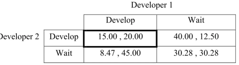
A numerical example is illustrated as followed. Using the same assumptions as presented in section 2.1.1, in a given city, the volatility of the asset value of office buildings is 20% and the growth rate of the construction or replacement cost is 5%. At t=0, the asset value of office building is $100 per sq.ft. while the construction cost is $70 per sq.ft. The risk-free rate is assumed to be 5%. In this city, assuming office developer 1 is a stronger developer and is better able to capture the market demand if it competes with office developer 2, then ωD1 will be bigger than ωD2. In this example, ωD1 is 0.9 and ωD2 is 0.85.
In this market, there is also a clear First Mover Advantage (FMA) because of the obvious, but finite, office demand. That implies that whoever develops first will benefit from the market condition. Therefore, ωLi will be bigger than ωDi, and in turn, ωDi will be
bigger than ωFi. Since developer 1 is a stronger player than developer 2, it can be
assumed that ωL1 is 1.15, ωL2 is 1.1, while ωF1 is 0.8, and ωF2 is 0.75. Using the real
options valuation model presented in 2.1.1 to calculate Ct1, Ct2, Ct1fwand Ct2fw, where Cti is
the option value of waiting for developer i when both developers wait and Ctifw is the
option value of waiting for developer i when developer i waits while the other developer develops ( = max (ωF1 St+1 – Kt+1e-r(t+1) , e-r(t+1) [q Cu(t+1)1fw + (1-q) Cd(t+1)1fw ] ), the game
theory payoff matrix is shown as follows:
Developer 1
Developer 2
Develop Wait
Develop 15.00 , 20.00 40.00 , 12.50
Wait 8.47 , 45.00 30.28 , 30.28
Table 2.3: Numerical Example Game Payoff Matrix Result
As the payoff matrix shows, the equilibrium between developer 1 and developer 2 is that they will develop together. This market is as depicted in Scenario 1: Develop-Develop Equilibrium. It is a classic Prisoner’s Dilemma situation. In this case, the game theory
explains why developers still choose to develop even though their option value of waiting is actually higher.
As illustrated above, the intrinsic values of ωDi, ωLi, and ωFi shape different market
conditions. Together with the option value of waiting, which is largely influenced by the volatility of asset value in certain given markets, the game matrix creates a rich
framework to analyze the timing strategy of real estate development at a strategic level. However, real-world situations are usually more complex than this simplified model. A few previous works by Grenadier (1996), Trigeorgis (1996) and Schwartz and Torous (2007) study some aspects of this option-game theoretic approach. It is particularly insightful to see how competitions erode option values and create a force to switch Wait-Wait Equilibrium as indicated in scenario 3 to Develop-Develop Equilibrium. In the next section, a more comprehensive and in-depth review will be presented to show how previous works have contributed to the development and understanding of the real options valuation and the game theory, particularly in the context of real estate development.
3.0 Chapter 3: Literature review
3.1 Real Options in Real Estate Development
Since the 1980s, there has been much interest in academic research about real options valuation methods and game theory application in the business world. A vast array of models and frameworks have been studied and proposed. Option theory was first applied to real estate by Titman (1985). “Urban Land Prices under Uncertainty” by Titman (1985) provides a valuation model for pricing vacant lots in urban areas. An implication of this relationship between uncertainty and vacant land values is that increased
uncertainty leads to a decrease in building activity in the current period. This model also provides insights into the role of real estate speculators who purchase vacant lots, and rather than develop them immediately, choose to keep them vacant for a period of time. The framework developed in this paper can also be extended to analyze other issues relating to real estate pricing under uncertainty. For example, it can be used to determine optimal time to demolish smaller building for redevelopment, and be used to analyze the effect of uncertainty on the optimal durability of buildings. This paper applies option valuation methods developed by Black and Scholes (1973) and Merton (1973). “Real Estate Development as an Option” by Williams (1991) solves the option pricing problem analytically and numerically for the optimal date and density of development, the optimal date of abandonment, and the resulting market values of the developed and undeveloped properties. “Mixed-Uses and the Redevelopment Option.” by Childs, P. D., Riddiough, T., and Triantis, A. J. (1995) considers how the potential for mixing uses and
redevelopment impact property value. Operating flexibility of this type is found to
significantly increase property value when the correlation between payouts from different property types is low or when redevelopment costs are low. The ability to mix uses and redevelop over time is also shown to affect the timing of initial land development.
3.2 Empirical Testing of Real Options Models in Real Estate Development
Until Quigg (1993), there had not been much empirical studies of real option models in real estate development. “Empirical Testing of Real Option-Pricing Models” by Quigg, L. (1993) examines the empirical predictions of a real option-pricing model using a large sample of market prices. She finds empirical support for a model that incorporates the option to wait to develop land. The option model has explanatory power for predicting transactions prices over and above the intrinsic value. Market prices reflect a premium for the option to wait to invest that has a mean value of 6% in their sample. She also
estimates the implied standard deviations for individual commercial property prices ranging from 18 to 28% per years. “Uncertainty and the Rate of Commercial Real Estate Development.” by Holland, S., Ott, S., and Riddiough, T. (1995) empirically examines the relationship between uncertainty and investment using commercial real estate data. To sort out long- versus short-run effects of asset volatility on investment decisions, they extend the standard real options model to determine the probability of investment over a particular time horizon. In doing so, they find that an increase in asset volatility can either increase or decrease the probability of development, although the anticipated negative short-run relationship is confirmed when the land is “ripe” for development (i.e., near the development hurdle value). The role of uncertainty in determining the rate of real
investment is then tested using aggregate data. By developing two measures of property value volatility, they empirically confirm the expected strong relationship between changes in uncertainty and the rate of development activity. “Effects of Uncertainty on the Investment Decision: An Examination of the Option-Based Investment Model Using Japanese Real Estate.” by Yoshida, J. (1999) examines the validity of the option-based investment model as opposed to the neoclassical investment model in the decision-making of commercial real estate development, using aggregate real estate data from Japan, focusing on the effect of uncertainty. It concludes that various kinds of real options must be incorporated in investment and economic models. “Empirical Testing of Real Option-Pricing Models Using Land Price Index in Japan.” by Yamazaki, R. (2000) examines the way uncertainty plays a role in built land prices. This paper provides basic
in this research analyzes micro land prices covering individual lot data provided by the Land Price Index. Since land prices are determined by both macro economic environment and micro lot-specific attributes, this paper utilizes both time-series economic data and cross-sectional (micro) data including uncertainty terms. In addition to the total
uncertainty in asset prices, this research also gives some ideas of cross-sectional
uncertainty in land price variations by utilizing cross-sectional amenity variables. These cross-sectional and time-series variables including these two uncertainty variables are pooled and the Ordinary Least Squares method is conducted. The results from the option-based models favor the application of the real option theory in land prices. The total uncertainty with respect to built asset return has a substantial effect on increasing land prices, which implies that an increase in uncertainty leads to an increase in land prices.
3.3 Game Theory in Real Estate Development
With the real options theory studied extensively as applied to real estate development and the business world in general, scholars started to question its incomplete application and limitation. Strategic interaction seems to have huge implication of the explanatory power of the real options model. That is how game theory is used to extend the real options model. “The Strategic Exercise of Options: Development Cascades and Overbuilding in Real Estate Markets” by Grenadier, S. R. (1996) develops an equilibrium framework for strategic option exercise games. He focuses on a particular example: the timing of real estate development. An analysis of the equilibrium exercise policies of developers provides insights into the forces that shape market behavior. The model isolates the factors that make some markets prone to bursts of concentrated development. The model also provides an explanation for why some markets may experience building booms in the face of declining demand and property values. While such behavior is often regarded as irrational overbuilding, the model provides a rational foundation for such exercise patterns. “Option Exercise Games: An Application to the Equilibrium Investment Strategies of Firms.” by Grenadier, S. R. (2000) provides a very general and tractable solution approach for deriving the equilibrium investment strategies of firms in a continuous-time Cournot-Nash framework. The impact of competition on exercise
strategies is dramatic. For example, while standard real options models emphasize that a valuable “option to wait” leads firms to invest only at large positive NPV, the impact of competition drastically erodes the value of the option to wait and leads to investment at very near the zero NPV threshold. The Nash equilibrium exercise strategies are shown to display the useful property that they are equivalent to those derived in an “artificial” perfectly competitive industry under a modified demand curve. This transformation permits a simplified solution approach for the inclusion of various realistic features into the model, such as time-to-build. “An Equilibrium Analysis of Real Estate Leases” by Grenadier, S. R. (2003) provides a unified equilibrium approach to valuing a wide variety of commercial real estate lease contracts. Using a game-theoretic variant of real options analysis, the underlying real estate asset market is modeled as a continuous-time Nash equilibrium in which developers make construction decisions under demand uncertainty. Then, using the economic notion that leasing simply represents the purchase of the use of the asset over a specified time frame, it uses a contingent-claims approach to value many of the most common real estate leasing arrangements. “Investment Under Uncertainty and Time-Inconsistent Preferences” by Grenadier, S. R., and Wang, N. (2006) extends the real options framework to model the investment timing decisions of entrepreneurs with such time-inconsistent preferences; developers are very impatient about choices in the short-term, but are quite patient when choosing between long-term alternatives. Two opposing forces determine investment timing: while evolving uncertainty induces entrepreneurs to defer investment in order to take advantage of the option to wait, their inconsistent preferences motivate them to invest earlier in order to avoid the time-inconsistent behavior they will display in the future. They find that the precise trade-off between these two forces depends on such factors as whether entrepreneurs are
sophisticated or naïve in their expectations regarding their future time-inconsistent behavior, as well as whether the payoff from investment occurs all at once or over time. They extend the model to consider equilibrium investment behavior for an industry comprised of time-inconsistent entrepreneurs. Such an equilibrium involves the dual problem of entrepreneurs playing dynamic games against competitors as well as against their own future selves. “Real Options and Games: Competition, Alliances and Other
the use of real options valuation and game theory principles to analyze prototypical investment opportunities involving important competitive / strategic decisions under uncertainty. It uses examples from innovation cases, alliances and acquisitions to discuss strategic and competitive aspects, relevant in a range of industries like consumer
electronics and telecom. It particularly focuses on whether it is optimal to compete independently or coordinate / collaborate via strategic alliances. “Commercial Office Space: Tests of a Real Options Model with Competitive Interactions.” by Schwartz, E. S., and Torous, W. N. (2007) tests a real options model with competitive interactions using an extensive commercial real estate data base. The competitive nature of the local real estate market as proxied by the market’s Herfindahl ratio is found to have a significant effect on building starts: larger values of the Herfindahl ratio, consistent with less competition, are associated with fewer building starts. In particular, a one standard deviation increase in this ratio leads to a 25.9% decreases in the number of new building starts. Other variables suggested by the real options model, such as the volatility of local lease rates, are also found to be important. “Irreversible investment, real options, and competition: Evidence from real estate development.” by Bulan, L., Mayer, C., and Somerville, C. (2008) examines the extent to which uncertainty delays investment, and the effect of competition on this relationship, using a sample of 1214 condominium developments in Vancouver, Canada built from 1979 to1998. They find that increases in both idiosyncratic and systematic risk lead developers to delay new real estate
investments. Empirically, a one-standard deviation increase in the return volatility reduces the probability of investment by 13 percent, equivalent to a 9 percent decline in real prices. Increases in the number of potential competitors located near a project negate the negative relationship between idiosyncratic risk and development. These results support models in which competition erodes option values and provide clear evidence for the real options framework over alternatives such as the neoclassical NPV valuation method.
3.4 Land Value Studies
“Insights on the Effect of Land Use Choice: The Perpetual Option on the Best of Two Underlying Assets” by Geltner, D., Riddiough, T. and Stojanovic, S (1996) considers the effect of land use choice on speculative land value and on development timing as
reflected in the optimal “hurdle ratio” which triggers immediate development. They found that land use choice may add over 40 percent to land value under typical economic circumstances. The conditions for optimal development of the land become markedly more difficult to achieve when the two land uses have similar values. In fact,
development will never occur when the two land use choices have equal value. “Swings in Commercial and Residential Land Prices in the United States” by Mulhall, M.,
Nichols, J., and Oliner, S. (2012) uses a large dataset of land sales dating back to the mid-1990s to construct land price indexes for 23 MSAs in the United States and for the aggregate of those MSAs. The price indexes show a dramatic increase in both
commercial and residential land prices over several years prior to their peak in 2006-07 and a steep descent since then. These fluctuations have exceeded those in well-known indexes of home prices and commercial real estate prices. Because those indexes price a bundle of land and structures, this comparison implies that land prices have been more volatile than structures prices over this period. This result is a key element of the land leverage hypothesis, which holds that home prices and commercial property prices will be more volatile, all else equal, in areas where land represents a larger share of real estate value.
4.0 Chapter 4: Methodology & Data Collection
4.1 Commercial Real Estate Asset and Land Value DataAsset values of 4 property types (Apartment, Industrial, Office, and Retail) in 30 Metropolitan Statistical Areas (MSA) spanning from 2001 to 2013 are collected from Real Capital Analytics, Inc (RCA) for the commercial portion of the study. The
construction or replacement cost data spanning from 1993 to 2013 is collected from RS Means. The residual land value is defined as the difference between the asset value and the construction or replacement cost. For the commercial portion, the construction activity is measured by number of square feet completed (industrial, office, and retail) and number of units completed (apartment), with data collected from CBRE.
The volatility (σ) of value or cost is calculated using historical data with the following equations:
ΔS = ln(! !!
!!!.!")
SD = (!!!!!!)!
σ = SD x 4 (annualized volatility for quarterly data)
4.1.1 Use of Real Capital Analytics (RCA) data
The RCA asset value data is transaction-based, not appraisal-based, and it is based on independent reports of properties and portfolios $2.5 million and greater. Quarterly non-smoothed data from 2001 to 2013 is used in the analysis of this paper.
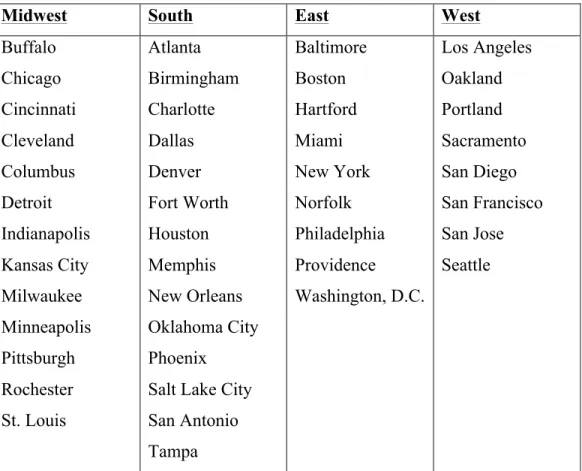
4.1.2 Comparison between 30 Metropolitan Statistical Areas (MSAs)
Midwest South East West
Chicago Atlanta Baltimore Los Angeles
Cincinnati Charlotte Boston Portland
Cleveland Dallas Miami San Diego
Columbus Denver New York San Francisco
Detroit Houston Philadelphia San Jose
Indianapolis Memphis Washington, D.C. Seattle
Kansas City Phoenix
Minneapolis Tampa
Pittsburgh St. Louis
Table 4.0: 30 Metropolitan Statistical Areas for Commercial Markets Analysis
Regarding the commercial markets, in general, RCA data shows that major U.S. cities such as Los Angeles, Washington DC, New York, and Boston are less volatile and less speculative than other second-tier or third-tier cities such as Pittsburgh, Detroit,
Memphis, and St Louis. Overall, the volatility of the West region is the lowest and the Midwest region is the highest. RCA data demonstrates higher volatility than expected, which is probably due to idiosyncratic variations of the transaction-based data. However, for the purpose of this thesis, which studies the timing strategy of developers, transaction-based data with higher volatility across all MSAs and property types is still consistent enough to be used for comparison purposes.
Regarding the land cost ratio, it is defined as the ratio of the residual land value to the asset value. RCA data demonstrates that the asset value volatility is negatively correlated with the land cost ratio. In other words, cities such as Washington DC, New York, San Francisco, and Boston with low volatility have high land cost ratios. Cities such as
section 5.0, the relationship between these variables and the timing strategy will be discussed empirically.
4.1.3 Comparison between 4 property types
Among the 4 property types (Apartment, Industrial, Office, and Retail), RCA data shows that the asset value volatility of office buildings is the lowest, followed by industrial buildings and retails. Apartment buildings have the highest volatility. For the office market, the East and West regions have the lowest volatility, while the Midwest region has the highest volatility. For the apartment and retail markets, the South and West regions have the lowest volatility, while the Midwest region again has the highest volatility. For the industrial market, the South and West regions again have the lowest volatility, while the East region has the highest volatility.
Regarding the land cost ratio, for the office and apartment markets, the East region has the highest land cost ratio, followed by the West and South regions. The Midwest region has the lowest land cost ratio. For the retail market, the West region has the highest land cost ratio, followed by the East and South regions. The Midwest region again has the lowest land cost ratio. For the industrial market, the East region has the lowest land cost ratio. At the property type aggregate level, the data again shows that the asset value volatility is negatively correlated with the land cost ratio. Office buildings demonstrate the lowest volatility and high land cost ratios. Apartment buildings have the highest volatility and low land cost ratios. It is also true at the regional level, the East region has the lowest volatility, but the highest land cost ratio, for the office market. The regression analyses yield the following results:
σ = α + β (LCR)
Where: σ = Asset Value Volatility
α = (P-value) β = (P-value) Overall 1.13 (4.59 x 10-49) -0.0377 (6.37 x 10⁻¹) Apartment 1.26 (1.79 x 10⁻¹⁴) -0.119 (5.16 x 10⁻¹) Industrial 1.14 (6.49 x 10⁻¹⁰) 0.186 (2.84 x 10⁻¹) Office 1.23 (5.59 x 10⁻¹³) -0.623 (5.17 x 10⁻³) Retail 1.38 (1.88 x 10⁻⁹) -0.426 (1.65 x 10⁻¹)
Table 4.1: Volatility and Land Cost Ratio Regression Results for Commercial Markets
With the results shown above, overall, except for the industrial market, the volatility is statistically negatively correlated with the land cost ratio:
!! !"#$ < 0
However, they are only weakly correlated, as indicated by the high P-values. The office market seems to be the only exception. Nonetheless, for any given MSA and property type, except for the industrial market, if the land value constitutes a small portion of the asset value, that asset type in that given market tends to be more volatile and relatively riskier to develop. The relationship between the volatility and the land cost ratio across 30 MSAs and 4 property types is summarized below: