Sampling
Population (Universe)
Population means aggregate of all possible units. It need not be human population. It may be population of plants, population of insects, population of fruits, etc. Parameter
A summary measure that describes any given characteristic of the population is known as parameter. Population are described in terms of certain measures like mean, standard deviation etc. These measures of the population are called parameter and are usually denoted by Greek letters. For example, population mean is denoted by , standard deviation by σ and variance by σ2 .
Sample
A portion or small number of unit of the total population is known as sample.
All the farmers in a village(population) and a few farmers(sample)
All plants in a plot is a population of plants.
A small number of plants selected out of that population is a sample of plants.
Statistic
A summary measure that describes the characteristic of the sample is known as statisitic. Thus sample mean, sample standard deviation etc is statistic. The statistic is usually denoted by roman letter.
- sample mean
s – standard deviation
The statistic is a random variable because it varies from sample to sample. Sampling
Sampling technique
There are two ways in which the information is collected during statistical survey. They are
1. Census survey 2. Sampling survey Census
It is also known as population survey and complete enumeration survey. Under census survey the information are collected from each and every unit of the population or universe.
Sample survey
A sample is a part of the population. Information are collected from only a few units of a population and not from all the units. Such a survey is known as sample survey.
Sampling technique is universal in nature, consciously or unconsciously it is adopted in every day life.
For eg.
1. A handful of rice is examined before buying a sack.
2. We taste one or two fruits before buying a bunch of grapes.
3. To measure root length of plants only a portion of plants are selected from a plot. Need for sampling
The sampling methods have been extensively used for a variety of purposes and in great diversity of situations.
In practice it may not be possible to collected information on all units of a population due to various reasons such as
1. Lack of resources in terms of money, personnel and equipment. 2. The experimentation may be destructive in nature. Eg- finding out the
germination percentage of seed material or in evaluating the efficiency of an insecticide the experimentation is destructive.
3. The data may be wasteful if they are not collected within a time limit. The census survey will take longer time as compared to the sample survey. Hence for getting quick results sampling is preferred. Moreover a sample survey will be less costly than complete enumeration.
4. Sampling remains the only way when population contains infinitely many number of units.
5. Greater accuracy. Sampling methods
The various methods of sampling can be grouped under 1) Probability sampling or random sampling
2) Non-probability sampling or non random sampling Random sampling
Under this method, every unit of the population at any stage has equal chance (or) each unit is drawn with known probability. It helps to estimate the mean, variance etc of the population.
Under probability sampling there are two procedures
1. Sampling with replacement (SWR)
2. Sampling without replacement (SWOR)
When the successive draws are made with placing back the units selected in the preceding draws, it is known as sampling with replacement. When such replacement is not made it is known as sampling without replacement.
When the population is finite sampling with replacement is adopted otherwise SWOR is adopted.
Mainly there are many kinds of random sampling. Some of them are.
1. Simple Random Sampling
2. Systematic Random Sampling
3. Stratified Random Sampling 4. Cluster Sampling
Simple Random sampling (SRS)
The basic probability sampling method is the simple random sampling. It is the simplest of all the probability sampling methods. It is used when the population is homogeneous.
Questions
1. If each and every unit of population has equal chance of being included in the sample, it is known as
(a) Restricted sampling (b) Purposive sampling
(c) Simple random sampling (d) None of the above
Ans: Simple random sampling
2.In a population of size 10 the possible number of samples of size 2 will be
(a) 45 (b) 40 (c) 54 (d) None of the above
Ans: 45
3.A population consisting of an unlimited number of units is called an infinite population.
Ans: True
4. If all the units of a population are surveyed it is called census. Ans: True
5. Random numbers are used for selecting the samples in simple random sampling method.
Ans: True
6. The list of all units in a population is called as Frame. Ans: True
7. What is sampling?
8. Explain the Lottery method.
9. Explain the method of selection of samples in simple random sampling. 10. Explain the method of selection of samples in Stratified random sampling.
Lecture.8
Test of significance Hypothesis
Hypothesis is a statement or assumption that is yet to be proved. Statistical Hypothesis
When the assumption or statement that occurs under certain conditions is formulated as scientific hypothesis, we can construct criteria by which a scientific hypothesis is either rejected or provisionally accepted. For this purpose, the scientific hypothesis is translated into statistical language. If the hypothesis in given in a statistical language it is called a statistical hypothesis.
For
eg:-The yield of a new paddy variety will be 3500 kg per hectare – scientific hypothesis.
In Statistical language if may be stated as the random variable (yield of paddy) is distributed normally with mean 3500 kg/ha.
Simple Hypothesis
When a hypothesis specifies all the parameters of a probability distribution, it is known as simple hypothesis. The hypothesis specifies all the parameters, i.e µ and σ of a normal distribution.
Eg:-The random variable x is distributed normally with mean µ=0 & SD=1 is a simple hypothesis. The hypothesis specifies all the parameters (µ & σ) of a normal distributions.
Composite Hypothesis
If the hypothesis specific only some of the parameters of the probability distribution, it is known as composite hypothesis. In the above example if only the µ is specified or only the σ is specified it is a composite hypothesis.
Null Hypothesis - Ho
Consider for example, the hypothesis may be put in a form ‘paddy variety A will give the same yield per hectare as that of variety B’ or there is no difference between the average yields of paddy varieties A and B. These hypotheses are in definite terms. Thus these hypothesis form a basis to work with. Such a working hypothesis in known as null hypothesis. It is called null hypothesis because if nullities the original hypothesis, that variety A will give more yield than variety B.
The null hypothesis is stated as ‘there is no difference between the effect of two treatments or there is no association between two attributes (ie) the two attributes are independent. Null hypothesis is denoted by Ho.
Eg:-There is no significant difference between the yields of two paddy varieties (or) they give same yield per unit area. Symbolically, Ho: µ1=µ2.
Alternative Hypothesis
When the original hypothesis is µ1>µ2 stated as an alternative to the null hypothesis is known as alternative hypothesis. Any hypothesis which is complementary to null hypothesis is called alternative hypothesis, usually denoted by H1.
Eg:-There is a significance difference between the yields of two paddy varieties. Symbolically,
H1: µ1≠µ2 (two sided or directionless alternative)
If the statement is that A gives significantly less yield than B (or) A gives significantly more yield than B. Symbolically,
H1: µ1 < µ2 (one sided alternative-left tailed) H1: µ1 > µ2 (one sided alternative-right tailed)
Sampling Distribution
By drawing all possible samples of same size from a population we can calculate the statistic, for example, for all samples. Based on this we can construct a frequency distribution and the probability distribution of . Such probability distribution of a statistic is known a sampling distribution of that statistic. In practice, the sampling distributions can be obtained theoretically from the properties of random samples.
Standard Error
As in the case of population distribution the characteristic of the sampling distributions are also described by some measurements like mean & standard deviation. Since a statistic is a random variable, the mean of the sampling distribution of a statistic is called the expected valued of the statistic. The SD of the sampling distributions of the statistic is called standard error of the Statistic. The square of the standard error is known as the variance of the statistic. It may be noted that the standard deviation is for units whereas the standard error is for the statistic.
Once the hypothesis is formulated we have to make a decision on it. A statistical procedure by which we decide to accept or reject a statistical hypothesis is called testing of hypothesis.
Sampling Error
From sample data, the statistic is computed and the parameter is estimated through the statistic. The difference between the parameter and the statistic is known as the sampling error. Test of Significance
Based on the sampling error the sampling distributions are derived. The observed results are then compared with the expected results on the basis of sampling distribution. If the difference between the observed and expected results is more than specified quantity of the standard error of the statistic, it is said to be significant at a specified probability level. The process up to this stage is known as test of significance.
Decision Errors
By performing a test we make a decision on the hypothesis by accepting or rejecting the null hypothesis Ho. In the process we may make a correct decision on Ho or commit one of two kinds of error.
We may reject Ho based on sample data when in fact it is true. This error in decisions is known as Type I error.
We may accept Ho based on sample data when in fact it is not true. It is known as Type II error.
Accept Ho Reject Ho
Ho is true Correct Decision Type I error
Ho is false Type II error Correct Decision
The relationship between type I & type II errors is that if one increases the other will decrease. The probability of type I error is denoted by α. The probability of type II error is denoted by β. The correct decision of rejecting the null hypothesis when it is false is known as the power of the test. The probability of the power is given by 1-β.
Critical Region
The testing of statistical hypothesis involves the choice of a region on the sampling distribution of statistic. If the statistic falls within this region, the null hypothesis is rejected: otherwise it is accepted. This region is called critical region.
true. Based on sample data it may be observed that statistic follows a normal distribution given by
We know that 95% values of the statistic from repeated samples will fall in the range
±1.96 times SE . This is represented by a diagram.
Region of Region of
rejection rejection
Region of acceptance
-1.96 0 1.96
The border line value ±1.96 is the critical value or tabular value of Z. The area beyond the critical values (shaded area) is known as critical region or region of rejection. The remaining area is known as region of acceptance.
If the statistic falls in the critical region we reject the null hypothesis and, if it falls in the region of acceptance we accept the null hypothesis.
In other words if the calculated value of a test statistic (Z, t, χ2 etc) is more than the critical value in magnitude it is said to be significant and we reject Ho and otherwise we accept Ho. The critical values for the t and are given in the form of readymade tables. Since the criticval values are given in the form of table it is commonly referred as table value. The table value depends on the level of significance and degrees of freedom.
Example: Z cal < Z tab -We accept the Ho and conclude that there is no significant difference between the means.
Test Statistic
The sampling distribution of a statistic like Z, t, & χ2
are known as test statistic. Generally, in case of quantitative data
Level of Significance
nothing but the probability of committing type I error. Technically the probability of committing type I error is known as level of Significance.
One and two tailed test
The nature of the alternative hypothesis determines the position of the critical region. For example, if H1 is µ1≠µ2 it does not show the direction and hence the critical region falls on either end of the sampling distribution. If H1 is µ1 µ2 or µ1 > µ2 the direction is known. In the first case the critical region falls on the left of the distribution whereas in the second case it falls on the right side.
Degrees of freedom
The number of degrees of freedom is the number of observations that are free to vary after certain restriction have been placed on the data. If there are n observations in the sample, for each restriction imposed upon the original observation the number of degrees of freedom is reduced by one.
The number of independent variables which make up the statistic is known as the degrees of freedom and is denoted by (Nu).
Steps in testing of hypothesis
The process of testing a hypothesis involves following steps. 1. Formulation of null & alternative hypothesis.
2. Specification of level of significance.
3. Selection of test statistic and its computation.
4. Finding out the critical value from tables using the level of significance, sampling distribution and its degrees of freedom.
5. Determination of the significance of the test statistic.
6. Decision about the null hypothesis based on the significance of the test statistic. 7. Writing the conclusion in such a way that it answers the question on hand.
Large sample theory
The sample size n is greater than 30 (n≥30) it is known as large sample. For large samples the sampling distributions of statistic are normal(Z test). A study of sampling distribution of statistic for large sample is known as large sample theory.
Small sample theory
If the sample size n ils less than 30 (n<30), it is known as small sample. For small
samples the sampling distributions are t, F and χ2 distribution
.
A study of sampling distribution for small samples is known as small sample theory.Test of Significance
The theory of test of significance consists of various test statistic. The theory had been developed under two broad heading
1. Test of significance for large sample
Large sample test or Asymptotic test or Z test (n≥30) 2. Test of significance for small samples(n<30)
Small sample test or Exact test-t, F and χ2.
It may be noted that small sample tests can be used in case of large samples also. 9 Small sample test
Student’s t test
When the sample size is smaller, the ratio will follow t distribution
and not the standard normal distribution. Hence the test statistic is given as
which follows normal distribution with mean 0 and unit standard deviation. This follows a t distribution with (n-1) degrees of freedom which can be written as t(n-1) d.f.
This fact was brought out by Sir William Gossest and Prof. R.A Fisher. Sir William Gossest published his discovery in 1905 under the pen name Student and later on developed and extended by Prof. R.A Fisher. He gave a test known as t-test.
Applications (or) uses
1. To test the single mean in single sample case.
(i) Independent samples(Independent t test) (ii) Dependent samples (Paired t test)
3. To test the significance of observed correlation coefficient.
4. To test the significance of observed partial correlation coefficient. 5. To test the significance of observed regression coefficient.
Test for single Mean 1. Form the null hypothesis
Ho: µ=µo
(i.e) There is no significance difference between the sample mean and the population mean
2. Form the Alternate hypothesis H1: µ≠µo (or µ>µo or µ<µo)
ie., There is significance difference between the sample mean and the population mean
3.Level of Significance
The level may be fixed at either 5% or 1% 4.Test statistic
which follows t distribution with (n-1) degrees of freedom
6. Find the table value of t corresponding to (n-1) d.f. and the specified level of significance.
7. Inference
If t < ttab we accept the null hypothesis H0. We conclude that there is no significant difference sample mean and population mean
(or) if t > ttab we reject the null hypothesis H0. (ie) we accept the alternative hypothesis and conclude that there is significant difference between the sample mean and the population mean.
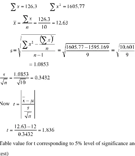
Based on field experiments, a new variety of green gram is expected to given a yield of 12.0 quintals per hectare. The variety was tested on 10 randomly selected
farmer’s fields. The yield (quintals/hectare) were recorded as
14.3,12.6,13.7,10.9,13.7,12.0,11.4,12.0,12.6,13.1. Do the results conform to the expectation?
Solution
Null hypothesis H0: =12.0
(i.e) the average yield of the new variety of green gram is 12.0 quintals/hectare. Alternative Hypothesis: H1:≠ 12.0
(i.e) the average yield is not 12.0 quintals/hectare, it may be less or more than 12 quintals / hectare
Level of significance: 5 % Test statistic:
From the given data
= 1.0853
Now
Table value for t corresponding to 5% level of significance and 9 d.f. is 2.262 (two tailed test)
Inference t < ttab
We accept the null hypothesis H0
We conclude that the new variety of green gram will give an average yield of 12 quintals/hectare.
Note
Before applying t test in case of two samples the equality of their variances has to be tested by using F-test
or
is the variance of the second sample whose size is n2.
It may be noted that the numerator is always the greater variance. The critical value for F is read from the F table corresponding to a specified d.f. and level of significance Inference
F <Ftab
We accept the null hypothesis H0.(i.e) the variances are equal otherwise the variances are unequal.
Test for equality of two Means (Independent Samples)
Given two sets of sample observation x11,x12,x13…x1n , and x21,x22,x23…x2n of sizes n1 and n2 respectively from the normal population.
1. Using F-Test , test their variances (i) Variances are Equal
Ho:., µ1=µ2
H1 µ1≠µ2 (or µ1<µ2 or µ1>µ2) Test statistic
where the combined variance
The test statistic t follows a t distribution with (n1+n2-2) d.f. (ii) Variances are unequal and n1=n2
It follows a t distribution with
This statistic follows neither t nor normal distribution but it follows Behrens-Fisher d distribution. The Behrens – Fisher test is laborious one. An alternative simple method has been suggested by Cochran & Cox. In this method the critical value of t is altered as tw (i.e) weighted t
where t1is the critical value for t with (n1-1) d.f. at a dspecified level of significance and t2 is the critical value for t with (n2-1) d.f. at a dspecified level of significance and
Example 2
In a fertilizer trial the grain yield of paddy (Kg/plot) was observed as follows Under ammonium chloride 42,39,38,60 &41 kgs
Under urea 38, 42, 56, 64, 68, 69,& 62 kgs.
Find whether there is any difference between the sources of nitrogen? Solution
Ho: µ1=µ2 (i.e) there is no significant difference in effect between the sources of nitrogen. H1: µ1≠µ2 (i.e) there is a significant difference between the two sources
Level of significance = 5%
Before we go to test the means first we have to test their variances by using F-test. F-test
Ho:., σ12=σ22 H1:., σ12≠σ22
Ftab(6,4) d.f. = 6.16
F < Ftab
We accept the null hypothesis H0. (i.e) the variances are equal. Use the test statistic
where
The degrees of freedom is 5+7-2= 10. For 5 % level of significance, table value of t is 2.228
Inference: t <ttab
We accept the null hypothesis H0
We conclude that the two sources of nitrogen do not differ significantly with regard to the grain yield of padd
Example 3
The summary of the results of an yield trial on onion with two methods of propagation is given below. Determine whether the methods differ with regard to onion yield. The onion yield is given in Kg/plot.
Method I Method II
n1=12 n2=12
Solution
Ho:., µ1=µ2 (i.e) the two propagation methods do not differ with regard to onion yield. H1 µ1≠µ2 (i.e) the two propagation methods differ with regard to onion yield.
Level of significance = 5%
Before we go to test the means first we have to test their variability using F-test. F-test Ho: σ12=σ22 H1: σ12≠σ22 Ftab(11,11) d.f. = 2.82 F > Ftab
We reject the null hypothesis H0.we conclude that the variances are unequal. Here the variances are unequal with equal sample size then the test statistic is
where
The table value for
=
11 d.f. at 5% level of significance is 2.201 Inference:t<ttab
We accept the null hypothesis H0
We conclude that the two propagation methods do not differ with regard to onion yield. Example 4
The following data relate the rubber yield of two types of rubber plants, where the sample have been drawn independently. Test whether the two types of rubber plants differ in their yield.
Type I 6.21 5.70 6.04 4.47 5.22 4.45 4.84 5.84 5.88 5.82 6.09 5.59 6.06 5.59 6.74 5.55
Type II 4.28 7.71 6.48 7.71 7.37 7.20 7.06 6.40 8.93 5.91 5.51 6.36
Solution
Ho:., µ1=µ2 (i.e) there is no significant difference between the two rubber plants. H1 µ1≠µ2 (i.e) there is a significant difference between the two rubber plants. Level of significance = 5%
Here
n1=16 n2=12
Before we go to test the means first we have to test their variability using F-test. F-test
Ho:., σ12=σ22 H1:., σ12≠σ22
if
Ftab(11,15) d.f.=2.51 F > Ftab
We reject the null hypothesis H0. Hence, the variances are unequal.
Here the variances are unequal with unequal sample size then the test statistic
t1=t(16-1) d.f.=2.131
t2=t(12-1) d.f .=2.201
Inference: t>tw
We reject the null hypothesis H0. We conclude that the second type of rubber plant yields more rubber than that of first type.
Paired t test
In the t-test for difference between two means, the two samples were independent of each other. Let us now take particular situations where the samples are not independent.
In agricultural experiments it may not be possible to get required number of homogeneous experimental units. For example, required number of plots which are similar in all; characteristics may not be available. In such cases each plot may be divided into two equal parts and one treatment is applied to one part and second treatment to another part of the plot. The results of the experiment will result in two correlated samples. In some other situations two observations may be taken on the same experimental unit. For example, the soil properties before and after the application of industrial effluents may be observed on number of plots. This will result in paired observation. In such situations we apply paired t test.
Suppose the observation before treatment is denoted by x and the observation after treatment is denoted by y. for each experimental unit we get a pair of observation(x,y). In case of n experimental units we get n pairs of observations : (x1,y1), (x2,y2)…(xn,yn). In order to apply the paired t test we find out the differences (x1- y1), (x2-y2),..,(xn-yn) and denote them as d1, d2,…,dn. Now d1, d2…form a sample . we apply the t test procedure for one sample (i.e)
,
the mean may be positive or negative. Hence we take the absolute value as . The test statistic t follows a t distribution with (n-1) d.f.
Example 5
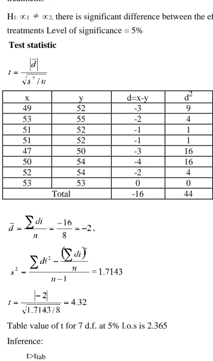
In an experiment the plots where divided into two equal parts. One part received soil treatment A and the second part received soil treatment B. each plot was planted with sorghum. The sorghum yield (kg/plot) was absorbed. The results are given below. Test the effectiveness of soil treatments on sorghum yield.
Soil treatment A 49 53 51 52 47 50 52 53
Soil treatment B 52 55 52 53 50 54 54 53
H0: 1 = 2 , there is no significant difference between the effects of the two soil treatments
H1: 1 ≠2, there is significant difference between the effects of the two soil treatments Level of significance = 5%
Test statistic x y d=x-y d2 49 52 -3 9 53 55 -2 4 51 52 -1 1 51 52 -1 1 47 50 -3 16 50 54 -4 16 52 54 -2 4 53 53 0 0 Total -16 44 ,
Table value of t for 7 d.f. at 5% l.o.s is 2.365 Inference:
We reject the null hypothesis H0. We conclude that the is significant difference between the two soil treatments between A and B. Soil treatment B increases the yield of sorghum significantly,