R E S E A R C H
Open Access
DOA estimation for periodically modulated
sources
Yi-Sheng Chen
Abstract
This paper considers the problem of direction-of-arrival estimation for periodically modulated signals using one uniform linear array of sensors. By means of modulating the sources with periodic modulation sequences, we can form a series of linear equations relating the autocorrelation matrices of the received data and the outer products of the scaled steering vectors. Solving these linear equations yields a group of Hermitian matrices formed from the outer products of the scaled steering vectors. Then taking the eigendecomposition of these Hermitian matrices, we can obtain all the scaled steering vectors. By utilizing a special structure of the scaled steering vectors, we can find the directions of signals impinging on the array. We also examine the relation of the modulation sequences and the estimation performance, and a design of the modulation sequences to resist the effect of spatial noise is proposed. One merit of the proposed method is that it can be used in the scenarios of more sources than sensors. The simulation result also shows that it has the capacity to distinguish the closely spaced sources.
Keywords: Direction-of-arrival, Uniform linear array, Periodic modulation
1 Introduction
The subject of array signal processing is concerned with the extraction of information from signals collected using an array (or arrays) of sensors [1,2]. One important infor-mation is the direction of arrival (DOA) of the incident signals. Take wireless communications for example, the information of DOA can be used for mobile localization for directional transmission in the downlink [3]. Hence, the DOA estimation of sources is one important research topic, and various algorithms in this field over the past decades have been proposed [1-7]. One of the famous algorithms is the multiple signal classification (MUSIC) algorithm proposed in [4]. The merit of the algorithm is that the accuracy of estimation can be obtained for large data samples or at high signal-to-noise ratio (SNR) scenarios. Another famous algorithm is the determinis-tic method developed by Van Der Veen [5]. Instead of requiring the statistical data and the search procedure in the angular spectrum inherently in the MUSIC algorithm, the deterministic method estimates the DOA directly in terms of eigenvalues of a certain matrix obtained from the received data. Due to the limitation of space, we cannot
Correspondence: [email protected]
Department of Communications Engineering, Feng Chia University, Taichung 40724, Taiwan
introduce all algorithms of DOA estimation, and we refer the interested readers to [1,2,7] and the references therein for a detailed review.
In digital communications, although the actual trans-mitted symbol stream is unknown to the receiver, some
a prioriinformation of the transmitted signals, for exam-ple, the modulation scheme, is available to the receiver. The receiver can take advantage of this extra information with the received data to carry out some tasks including source separation and channel estimation [8-11]. Partic-ularly in [9,10], the signal sources transmitted are first multiplied at a symbol rate by known amplitude-variation sequences, called modulation sequences, to aid symbol recovery or channel estimation at the receiver. However, there is little research for DOA estimation using modu-lation sequences. This motivates our research interest in developing a new DOA estimation method for one uni-form linear array (ULA) based on modulation sequences.
Our idea and method are shown as follows: By means of modulating the sources with periodic modulation sequences, we can form a set of autocorrelation matri-ces of the received data. Then the set of autocorrelation matrices allows us to formulate a series of linear equations relating the outer products of the scaled steering vectors. Solving the set of linear equations produces a group of
Hermitian matrices, which are the outer products of the scaled steering vectors. Then taking the eigendecompo-sition of these Hermitian matrices, we can obtain all the scaled steering vectors. By utilizing a special structure of the scaled steering vectors, we can find the direc-tions of signals impinging on the array. We also examine the relation of the modulation sequences and the esti-mation performance, and a design of the modulation sequences to resist the effect of spatial noise is proposed. The merit of the proposed method is that it can be used in the case of more sources than sensors. In addition, the method has the capacity to distinguish the closely spaced sources.
It is worth to mention that since the periodically modu-lated signals are artificial, the proposed method is suitable for communication signals. One possible application of the proposed method is mobile localization for directional transmission in the downlink since the modulation for-mats of the mobile units are available to the base station in the uplink [3,11].
This paper is organized as follows: Section 2 briefly reviews the system model and provides basic assumptions. In Section 3, we derive the estimation method and discuss some properties of the proposed algorithm. Simulation results are given in Section 4. Section 5 concludes this paper.
1.1 Notations
(·)∗,(·)T, and(·)H denote the complex conjugate, trans-pose, and conjugate transpose operations, respectively. The notation · 2is the 2-norm. The symbolsRandC represent the set of real numbers and the set of complex numbers, respectively.IMis the identity matrix of dimen-sionM×M.A◦Bis the Hadamard product of matricesA∈
Cm×nandB∈ Cm×n([12], p. 190), andA(:,k)andA(l, :) are thekth column vector and thelth row vector of A, respectively. For a vectorb∈Cm,b(r
1:r2)is the
subvec-tor formed from ther1th element to ther2th element ofb.
In addition, for anym×mmatrixG=[gk,l]0≤k,l≤m−1, we
define the operationj(G) = [g0,jg1,j+1· · ·gm−1−j,m−1]T,
for 0≤j≤m−1, i.e.,j(G)is the column vector formed from thejth superdiagonal ofG.
2 Problem statement
Consider a uniform linear array ofMsensors where adja-cent sensors are separated with equal distance d. The sensor array receives N narrowband sources from far-field whose directions of arrival are θ1, θ2,· · ·, andθN, respectively. Before transmission, each sourcesi(k),∀i = 1, 2,· · ·,N, is multiplied by a real and periodic modula-tion sequence ci(k). Then the standard system model is shown as follows:
y(k)=Asp(k)+w(k), (2.1)
where y(k) ∈ CM is the received vector at time k. A=[a(θ1)a(θ2)· · ·a(θN)]∈CM×N is the array response matrix with the ith column being the steering vector a(θi) = [ 1e−jφ(θi)e−j2φ(θi)· · · e−j(M−1)φ(θi)]T∈ CM of sourcei, whereφ(θi)= 2πdsinλ (θi) andλ≥2dis the signal wavelength.w(k)∈CMis the spatial noise vector at time
k.sp(k)∈CN is the transmitted vector defined as follows: sp(k) = [c1(k)s1(k)c2(k)s2(k)· · ·cN(k)sN(k)]T
= C(k)s(k), (2.2)
where C(k) = diag[c1(k)c2(k)· · ·cN(k)]∈ RN×N and s(k)=[s1(k)s2(k)· · ·sN(k)]T∈CN.
The purpose of this paper is to develop a method of estimatingθi fori = 1, 2,· · ·,N, using the second-order statistics of the received data based on the following assumptions:
(i) The source vectors(k)is a zero-mean, temporally and spatially uncorrelated, and wide-sense stationary vector withE[|si(k)|2]=d2i. The noise vectorw(k)is
zero-mean, wide-sense stationary, and
E[w(m)w(n)H]=σw2δ(m−n)IM, whereδ(·)is the
Kronecker delta function. In addition, the source signal is uncorrelated with the noise, i.e., E[s(m)w(n)H]=0,∀m,n.
(ii) The DOAθi ∈
−π2,π2,i=1, 2,· · ·,N. (iii) Each of the modulation sequencesci(k),
i=1, 2,· · ·,N, is periodic with periodP≥N+1, i.e.,ci(k)=ci(k+P).
3 DOA estimation
In this section, we first derive the estimation method when noise is absent. The design of the modulation sequences when noise is present is given in Section 3.2. Some further discussions about the proposed method are given in Section 3.3.
3.1 The proposed method
Using (2.2), the system model (2.1) for the noiseless case can be expressed as
y(k)=AC(k)s(k). (3.1)
Taking the expectation ofy(k)y(k)H fork =1, 2,· · ·,P
and using assumption (i), we obtain the followingP auto-correlation matrices:
Rk = E[y(k)y(k)H]
= AC(k)DC(k)AH, k=1, 2,· · ·,P, (3.2)
where D = diag[d12d22· · ·d2N]∈ RN×N. Since D and C(k)are real and diagonal matrices, (3.2) can be further expressed as
Rk = AD 1
2C(k)2D12AH
Here we let AD12 = H = [h1h2· · ·hN] with hi = dia(θi)be the scaled steering vector fori=1, 2,· · ·,N.
SinceC(k)is a diagonal matrix formed from the peri-odic modulation sequences c1(k),c2(k), · · ·,cN(k) with periodPby assumption (iii), we know thatC(k)2is also
periodic with periodP, i.e., C(k)2 = C(k+P)2, which
implies thatRk+P = Rk, for example, R1+P = R1. In
addition, for the purpose of DOA estimation, we need the following proposition to aid our derivation of the proposed method.
Proposition 1. For k=1, 2,· · ·,P, the ith upper diagonal ofRkcan be expressed as follows:
i(Rk)=
With the aid of Proposition 1, we obtain the vectors
i(R1),i(R2),· · ·,i(RP)from (3.4) to form a matrixVi be written as a linear equation shown as follows:
Vi(:,k)=WXi(:,k),k=1, 2,· · ·,M−i. (3.6)
Since P > N by assumption (iii), we can appro-priately design the modulation sequences {cn(1),cn(2),
· · ·,cn(P)},n=1, 2,· · ·,N, to make the matrixWbe full column rank. Then for eachi,i=0, 1,· · ·,M−1, the least squares solutions of (3.6) are shown as follows:
Xi(:,k)=(WTW)−1WTVi(:,k),k=1, 2,· · ·,M−i. (3.7)
Then each column ofXi, solved by (3.7), is used to form the matrixXi,∀i=0, 1,· · ·,M−1. Taking the transpose
ofXi, we obtainZisinceZi =XTi ,i=0, 1,· · ·,M−1. In addition, from (3.4), we know that
Zi=
By writing down the elements inZiwith the aid of the Hadamard product, we observe that
Zi = in (3.10) obtained from (3.7) allow us to form N rank-one Hermitian matricesQn = hnhHn, which is the outer product matrix ofhn,n=1, 2,· · ·,N. Then each column vectorhnofHis estimated up to a scalar ambiguityαnby computing the unit-norm eigenvector associated with the maximal eigenvalue of the matrixQn, i.e.,
hn=hnαn,n=1, 2,· · ·,N. (3.11)
Then we divide each scaled steering vector hn into two subvectors, namely hn1 = hn(1 : M − 1) and
hn2=hn(2 :M). It is clear thathn1=hn2ejφ(θn)andejφ(θn)
can be obtained from the least squares solution. Then the DOAθnis thus obtained from the angle ofejφ(θn).
3.2 The design of the modulation sequences
We have derived the estimation method in Section 3.1. We now discuss how to design the modulation sequences to combat the effect of noise on DOA estimation.
When noise is present, the system model (3.1) becomes y(k)=AC(k)s(k)+w(k) (3.13) and the autocorrelation matrices in (3.3) become
Rk = E[y(k)y(k)H]
= HC(k)2HH+σw2IM,k=1, 2,· · ·,P. (3.14) Since the noise variance only appears on the main diago-nal ofRk, the groups of vectorsi(Rk),i=1, 2,· · ·,M−1 in (3.4) remain unchanged, and only the group of vectors
0(Rk)needs to be changed as
Then the correspondingMlinear equations from (3.16) become
V0(:,k)=WX0(:,k)+σw21P,k=1, 2,· · ·,M. (3.17) From (3.7), we know that the solutions of (3.17) become
X0(:,k) = (WTW)−1WTV0(:,k)
wqdue to noise. Sinceqis formed from the modulation sequences, we need to design the modulation sequences to minimize q2 and the effect of the resulting per-turbation term. However, the high nonlinearity of the modulation sequences contained in q makes it difficult to design. Hence, we adopt another reasonable design criterion which is also used in [10] to tackle this problem. From (3.18), we know theX0(:,k)=X0(:,k)if and only can be selected to meet the orthogonality condition (3.19), the effect of noise is completely eliminated, but this is impossible since the entries ofw1,w2,· · ·,wNand1Pare
positive. Therefore, we seek to choose the modulation sequences such that1P is as close to being orthogonal to wias possible, fori = 1, 2,· · ·,N. To this end, we define and try to choose the modulation sequences to minimize the correlation coefficientγisubject to the following two constraints: the power gain of the modulation sequence of each source to 1, and constraint (3.22) requires that at each instant, the power gain is no less thanτ. Note that the optimization problem is identical to the case considered in [10], and the resulting optimal sequences are given by, for any fixed 1≤
mi≤P, mation using periodic modulation [10], the two-level sequence in (3.23) is also shown to be optimal for mitigating the channel noise effect. In addition, with the optimal solution in (3.23), the corresponding γi is
γopt = √ 1
P(1−τ)2+τ(2−τ), ∀i = 1, 2,· · ·,N. Note that γopt decreases as τ decreases, and thus, the noise effect imposed on V0is reduced and hence estimation
perfor-mance improves. We will give a simulation example to illustrate this property.
From (3.23), we know that each of theN modulation sequences is a two-level sequence with a single peak in one period. However, to make the matrixWbe full col-umn rank such that the least squares solutions (3.7) can be computed, the peak locations of the N modulation sequences in one period need to be distinct with one another, i.e., mk = ml for all k = l. Without loss of generality, we can letmi=ifori=1, 2,· · ·,N.
Remark 2.It is worth noting that even for the colored noise case, the design of modulation sequences is the same as the case of white noise. To see this, we know that if the zero-mean, wide-sense stationary noise vector w(k)
in assumption (i) now becomes colored, then theM×M
autocorrelation matrix Rw = E[w(k)w(k)H] becomes a Hermitian and Toeplitz matrix withi(Rw)=σw2(i)1M−i,
E[y(k)y(k)H]= HC(k)2HH +Rw, which means fori =
0, 1,· · ·,M−1,
i(Rk)=Zi
c1(k)2 c2(k)2 · · · cN(k)2
T+σ2
w(i)1M−i (3.24)
and
Vi=WXi+σw2(i)
1P1P· · ·1P
(M−i)columns
. (3.25)
The least squares solution of (3.25) is
Xi = (WTW)−1WTVi
= Xi+σw2(i)(WTW)−1WT
1P1P· · ·1P
(M−i)columns
. (3.26)
From (3.26), it is obvious that if WT1P =
w1 w2 · · · wN
T
1P =0, then the effect of noise can be eliminated. From here, the discussion and derivation are the same as the content from (3.19) to (3.23). Hence we know that the optimal sequences given in (3.23) can work well for the colored noise case. We will give a simulation in Section 4 to demonstrate this feature.
3.3 Discussions
We now discuss some notable features of the proposed method. First, from the result at the end of Section 3.1, we know that afterhnis estimated, the DOA angleθncan be obtained from the linear equationhn1 = hn2ejφ(θn).
Sincehn is an M× 1 vector, the DOA angleθn can be acquired provided thatM ≥ 2, whereMis the number of sensors for the ULA. Hence, the proposed method can carry out DOA etimation not only for the case of more sensors (M ≥ N), but also for the case of less sensors
(M < N), as long as the number of sensorsM ≥2. Sec-ond, the DOAθn ∈[−π2,π2],n =1, 2,· · ·,N, may not be distinct with each other since from Section 3.1, we know that the estimates ofθ1,θ2,· · ·, andθN are independently obtained from the corresponding scaled steering vectors
h1,h2, · · ·, andhN, respectively. Hence, the proposed
method possesses the capacity to distinguish the closely spaced sources. We will give a simulation to demonstrate this feature. The third feature of the proposed method is that it provides a design of the modulation sequences to minimize the effect of noise on DOA estimation and thus improves the accuracy of the solution.
We now summarize the proposed approach as the fol-lowing algorithm:
1. Collect the received data{y(m)}Sm=1, whereS divides P, the period of the modulation sequences.
2. Compute the autocorrelation matricesR1,R2,· · ·
RP, via the following time average:
Rk= 1
S/P S P−1
n=0
y(k+nP)y(k+nP)H,k=1, 2,· · ·,P.
(3.27)
3. Use the autocorrelation matrices in (3.27) to form
V0,V1,· · ·,VM−1, and use the designed modulation sequences (3.23) to formW.
4. Obtain the matricesX0,X1,· · ·,XM−1using the least squares solutions in (3.7) with the aid of the matricesV0,V1,· · ·,VM−1, andWobtained from the previous step.
5. FormN rank-one Hermitian matricesQ1,Q2,· · ·,
QNfromZi=XTi ,i=0, 1,· · ·,M−1, with the aid
of (3.10).
6. For eachQn=hnhHn, compute the estimatehnas
the unit-norm eigenvector associated with the maximal eigenvalue ofQn,∀n=1, 2,· · ·,N.
7. Divide each scaled steering vectorhninto two
subvectors, namelyhn1=hn(1 :M−1, :)and
hn2=hn(2 :M, :). Then obtain the DOA from the angle of the least squares solution of the linear equationhn1=hn2ejφ(θn).
4 Simulation
In this section, we use several simulations to demon-strate the performance of the proposed method. For all simulation examples, the SNR is defined as SNR =
Ey(k)−w(k)2 2
Ew(k)2 2
. We use the root-mean-square error
(RMSE) of angles as the performance measure, which
is defined as RMSE =
EN1Nn=1(θn−θn)2
, where
θn is the estimate of θn. The number of Monte Carlo trials is 500. The source symbols are independent and identically distributed binary phase-shift keying signals. The noise is zero-mean and white Gaussian (except for simulation 3).
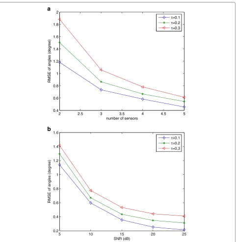
4.1 Simulation 1 - underdetermined DOA estimation
In this simulation, we execute two underdetermined experiments where the number of sensors is less than the number of sources. There are six signal sources in both experiments with the corresponding DOA:
{θ1,θ2,· · ·,θ6} = {−60◦,−45◦,−30◦, 30◦, 45◦, 60◦}. For both experiments, we setd=0.5λand we adopt the mod-ulation sequence ci(k)in (3.23) for source iwith period
2 2.5 3 3.5 4 4.5 5 0.4
0.6 0.8 1 1.2 1.4 1.6 1.8 2
number of sensors
RMSE of angles (degree)
τ=0.1
τ=0.2
τ=0.3
5 10 15 20 25
0.2 0.4 0.6 0.8 1 1.2 1.4 1.6
SNR (dB)
RMSE of angles (degree)
τ=0.1 τ=0.2 τ=0.3
a
b
Figure 1RMSE of angles for underdetermined cases.(a) SNR=10 dB. (b) Four sensors.
improves the performance of DOA estimation. This may be due to more information obtained to average out the computational error and noise effect for more sensors. In the second experiment, the ULA is only composed of four sensors. From Figure 1b, we observe that the RMSE of angles decreases as SNR increases. In addition, both experiments also show that the estimation performs bet-ter for smallerτ, which is consistent with our analysis in Section 3.2.
4.2 Simulation 2 - comparison with existing methods
In this simulation, we examine the performance of the proposed method with those of the conventional MUSIC algorithm [4] and the deterministic method [5] for two sources. The ULA is composed of five sensors withd =
0.5λ. For the proposed method, the modulation sequence
ci(k)for sourceiis chosen as in (3.23) with periodP=3,
nonclosely spaced sources:{θ1,θ2} = {−15◦, 15◦}. Simu-lation results in Figure 2a show that the proposed method performs better than both methods in [4,5] except for the deterministic method for SNR > 15 dB. Then we con-sider the case of two closely spaced sources:{θ1,θ2} =
{−15◦,−12◦}. Since the MUSIC algorithm fails to resolve the closely spaced signals under the simulation setting, we only compare the proposed method with the determinis-tic method. From Figure 2b, we observe that the proposed method performs better than the deterministic algorithm for this case. It also shows that the capacity of the pro-posed method to distinguish two closely spaced sources is good.
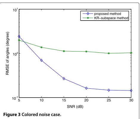
4.3 Simulation 3 - underdetermined DOA estimation in the presence of colored noise
In this simulation, we examine the performance of the proposed method with that of the Khatri-Rao (KR) sub-space method [6] for the colored noise case. The additive colored noisew(n) is generated by passing a zero-mean with unit variance white sequencewv(n)through a finite impulse response filterc(z)=1.2+0.6z−1+0.3z−2whose
output isw(n) = c(z)wv(n). Assume that there are four signal sources with{θ1,θ2,θ3,θ4} = {−60◦,−30◦, 30◦, 60◦} and the ULA is composed of three sensors withd=0.5λ. For the proposed method, the modulation sequenceci(k) for source i is chosen as in (3.23) with period P = 5,
τ =0.2, and peak locationmi =i,i= 1, 2, 3, 4. Since the KR subspace method is suitable for the quasi-stationary signals, we randomly choose the standard deviation of sig-nals following a uniform distribution on [ 0, 2√3] such that the variance is 1. In addition, 50 frames with each period being 100 are used to carry out the simulation for the KR subspace method. In other words, the number of symbol blocks isS = 5, 000. From Figure 3, we observe that the KR subspace results in better performance for SNR < 7 dB. However, for SNR > 7 dB, the proposed
5 10 15 20 25 30
10-1 100
101
SNR (dB)
RMSE of angles (degree)
proposed method KR−subspace method
Figure 3Colored noise case.
method achieves smaller RMSE of angles than that of the KR subspace method.
5 Conclusion
This paper has proposed a new DOA estimation algo-rithm for one ULA based on periodic modulation. The proposed method has three notable features. First, the proposed algorithm can handle more sources than sen-sors, which may be few as two. In addition, the great capacity to distinguish the closely spaced sources is the second feature of the proposed method. The final feature of the proposed method is that the performance of the estimation algorithm depends on the choice of the modu-lation sequences to resist the noise effects. Hence, we can properly choose the modulation sequences to improve the performance of estimation. Simulation results are used to demonstrate the performance of the proposed method and to compare it with some existing methods.
0 5 10 15 20 25 30
10-3 10-2
10-1 100
SNR (dB)
RMSE of angles (degree)
proposed method method in [4] method in [5]
(a)
5 10 15 20 25 30
10-2 10-1 100
101
102
SNR (dB)
RMSE of angles (degree)
proposed method method in [5]
(b)
Appendix
From the Preliminary, we know that (1) can be further expressed as
(2) asserts the result given in Proposition 1.
Competing interests
The author declares that he has no competing interests.
Acknowledgements
This research was sponsored by the National Science Council of Taiwan under grant NSC-99-2221-E035-056-.
Received: 23 May 2012 Accepted: 23 April 2013 Published: 24 May 2013
References
1. H Krim, M Viberg, Two decades of array signal processing. IEEE Signal Process. Mag.13(4), 67–94 (1996)
2. HL Van Trees,Optimal Array Processing. (Wiley, New York, 2002) 3. Veen Van Der A J, MC Vanderveen, AJ Paulraj, Joint angle and delay
estimation using shift-invariance properties. IEEE Signal Process. Lett. 4(5), 142–145 (1997)
4. RO Schmidt, Multiple emitter location and signal parameter estimation. IEEE Trans. Antennas Propagation.34(3), 276–280 (1986)
5. Veen Van Der A J, Algebraic methods for deterministic blind beamforming. Proc. IEEE.86(10), 1987–2008 (1998)
6. WK Ma, TH Hsieh, CY Chi, DOA estimation of quasi-stationary signals with less sensors than sources and unknown spatial noise covariance: a Khatri-Rao subspace approach. IEEE Trans. Signal Process. 58(4), 2168–2180 (2010)
7. Z Chen, G Gokeda, Y Yu,Introduction to Direction-of-Arrival Estimation. (Artech House, Norwood, 2010)
8. GB Giannakis, Y Hua, P Stoica, L Tong,Signal Processing Advances in Wireless and Mobile Communications, Volume II: Trends in Single- and
Multi-User Systems. (Prentice Hall PTR, Upper Saddle River, 2001)
9. R Djapic, Veen Van Der A J, L Tong, Synchronization and packet separation in wireless ad hoc networks by known modulus algorithms. IEEE J. Selected Areas Commun.23(1), 51–64 (2005)
10. CA Lin, JW Wu, Blind identification with periodic modulation: a time-domain approach. IEEE Trans. Signal Process.
50(11), 2875–2888 (2002)
11. J Li, B Halder, P Stoica, M Viberg, Computationally efficient angle estimation for known waveforms. IEEE Trans. Signal Process. 43(9), 2154–2163 (1995)
12. F Zhang,Matrix Theory: Basic Results and Techniques. (Springer, New York, 1999), p. 190
doi:10.1186/1687-6180-2013-110
Cite this article as: Chen:DOA estimation for periodically modulated sources.EURASIP Journal on Advances in Signal Processing20132013:110.
Submit your manuscript to a
journal and benefi t from:
7Convenient online submission 7 Rigorous peer review
7Immediate publication on acceptance 7 Open access: articles freely available online 7High visibility within the fi eld
7 Retaining the copyright to your article