Production Planning with Clearing Functions: Data-driven Approaches and Conic Programming.

(1)

Abstract

GOPALSWAMY, KARTHICK. Production Planning with Clearing Functions: Data-driven Approaches and Conic Programming (Under the direction of Reha Uzsoy).

In this dissertation, we study the production planning problem with clearing functions (PP-CF). PP-CF is important in theory and practice, as it combines the elegance of mathematical programming with the robustness of queuing theory to provide realistic models. A major component of PP-CF is estimating clearing functions from simulation data. We identify several issues associated with the resulting regression problem such as observation bias and restrictive functional form issues, provide a data-driven iterative refinement procedure to address the issue of observation bias. We tackle the functional form restriction by using a more generalized piecewise linear functional form based on the properties of the clearing functions and provide effective implementation of these functional forms in optimization. Numerical experiments are provided as an evidence of significant improvement in performance measures using iterative-refinement procedure. We then develop a method to provide effective fitting of piecewise linear clearing functions to simulation or empirical data using mixed integer linear programming (MILP). The new method uses a fixed number of linear segments to provide a globally optimal fit to the data using a piecewise linear concave function. It outperforms other known state-of-the-art linearization methods as supported by intensive computational experiments.

(2)

(3)

Production Planning with Clearing Functions: Data-driven Approaches and Conic Programming

by

Karthick Gopalswamy

A dissertation submitted to the Graduate Faculty of North Carolina State University

in partial fulfillment of the requirements for the Degree of

Doctor of Philosophy

Industrial Engineering

Raleigh, North Carolina

2019

APPROVED BY:

Yahya Fathi Michael Kay

Yunan Liu Haldun Aytug

External Member

Reha Uzsoy

(4)

Dedication

(5)

Biography

Karthick Gopalswamy was born in Kacheepuram, TamilNadu, India. He attended SSN College of Engineering (Affiliated to Anna University) in TamilNadu, India and received his Bachelor of Engineering degree in Mechanical Engineering in 2012. Later that year, he joined Larsen and Toubro as a graduate trainee and left the company as a Senior Engineer in 2014 to purse higher studies. He joined the Department of Industrial and Systems Engineering at NC State University and began pursuing his Ph.D. degree under the guidance of Dr. Reha Uzsoy. He was awarded a Master of Industrial Engineering degree in 2016 from the same institution. He held several teaching and research assistantship positions while at NC State.

(6)

Acknowledgements

This dissertation would not have been possible without the guidance of my committee members and the encouragement and support from my family and friends.

First and foremost, I would like to express my heartfelt and most sincere gratitude and appreciation to my advisor Dr. Reha Uzsoy. It has been an honor to work with him. I am thankful that he provided me with an excellent atmosphere for doing research. I appreciate his guidance, support, encouragement, patience, and sense of humor. I would also like to thank Dr. Michael G. Kay, who has been instrumental throughout my studies at NC State. His unique practical perspective on all aspects of academics as well as life in general has been invaluable to me. I am grateful to all my committee members for the enthusiasm they showed for my dissertation and the invaluable feedback they provided me throughout my research. I would like to thank Dr. Yahya Fathi for his help especially on valid inequalities and the derivation of proofs. My thanks also go to Dr. Yunan Liu for his insights on stochastic models and his queuing classes which helped me with the queueing perspective of this thesis. He has been my inspiration to stay fit both mentally and physically, while meeting the demands of doing a PhD.

I am indebted to many excellent people who have contributed to my education. I would like to thank all the faculty of Department of Industrial Engineering at NC State for their encouragement and support.

(7)

LIST OF TABLES

Table 3.1 Experimental Design. . . 32

Table 3.2 Friedman Test (p value) for mean difference comparison for Un-planned and Iterative algorithms with nonlinear CF. . . 36

Table 3.3 Friedman Test (p value) for mean difference comparison for Un-planned and Iterative algorithms with min-affine CF. . . 40

Table 3.4 Percentage decrease in average costs ofmin-affine CF over nonlinear CF. . . 40

Table 3.5 Average cost using nonlinear CF with b= 50, h= 15, w = 35. . . . 41

Table 3.6 Average cost usingmin-affine CF with seasonal demand,b= 50, h= 5, w = 6. . . 41

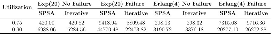
Table 3.7 Average cost comparison between Iterative and SPSA algorithms (min-affine CF), b= 50, h= 5, w = 6. . . 42

Table 4.1 Model comparison. . . 49

Table 4.2 Model comparison for univariate case n= 1. . . 51

Table 4.4 Summary of LP-bound GapobjIP_obj−IPobjLP% . . . 55

Table 4.5 Computation Time Summary for Test instances: m= 100. . . 56

Table 4.8 Optimality Gap Summary for Test Instances:m= 100. . . 57

Table 4.9 Optimality Gap Summary for Test Instances:m= 200. . . 57

Table 4.10 Optimality Gap Summary for Test Instances: m= 400. . . 58

Table 4.11 Summary of Number of Nodes explored for Test instances. . . 58

Table 4.12 Average solution time and optimality gap for p= 2 with large m. . 58

Table 5.1 Processing Time Distributions (lognormal distributed). . . 69

Table 5.2 Failure Distribution Parameters (minutes). . . 69

Table 5.4 Solution time comparison (in hrs). . . 73

Table 5.5 Intercepts of CF fit: Failure. . . 73

Table 5.6 Slopes of CF fit: Failure. . . 73

Table 5.7 Average cost comparison: No failure. . . 74

Table 5.8 Average cost comparison: Failure. . . 74

Table 5.9 Worst case cost comparison: No failure. . . 74

Table 5.10 Worst case cost comparison: Failure. . . 74

Table 6.2 Data parameters for the optimization model. . . 99

(10)

(11)

LIST OF FIGURES

Figure 1.1 Clearing function and Effect of Variability. . . 5

(a) Clearing function, Karmarkar (1989). . . 5

(b) Effect of Variability, Missbauer (2002). . . 5

Figure 2.1 Best case CF, Hopp & Spearman (2011). . . 16

Figure 3.1 A graphical visualization of CAP algorithm. . . 28

(a) Original Partition. . . 28

(b) k= 1, Mˆ112. . . 28

(c) k= 1, Mˆ111. . . 28

(d) k= 2, Mˆ122. . . 28

(e) k= 2, Mˆ121. . . 28

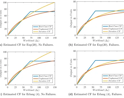
Figure 3.2 Performance of iterative fitting for nonlinear CF (6.5) of Karmarkar (1989). . . 34

(a) Estimated CF for Exp(20), No Failures. . . 34

(b) Estimated CF for Exp(20), Failures. . . 34

(c) Estimated CF for Erlang (4), No Failures. . . 34

(d) Estimated CF for Erlang (4), Failures. . . 34

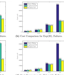
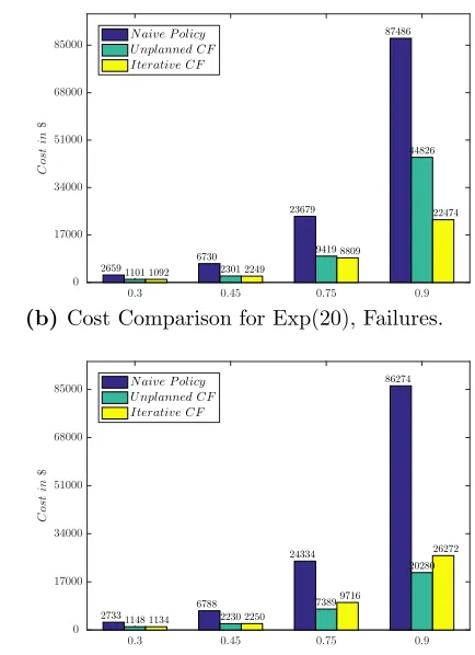
Figure 3.3 Graphs showing the cost distribution across different scenarios for nonlinear CF iterative procedure. . . 37

(a) Cost Comparison for Exp(20), No Failures. . . 37

(b) Cost Comparison for Exp(20), Failures. . . 37

(c) Cost Comparison for Erlang(4), No Failures. . . 37

(d) Cost Comparison for Erlang(4), Failures. . . 37

Figure 3.4 Performance of Iterative Fitting for piecewise linear CF. . . 39

(a) Cost Comparison for Exp(20), No Failures. . . 39

(b) Cost Comparison for Exp(20), Failures. . . 39

(c) Cost Comparison for Erlang(4), No Failures. . . 39

(d) Cost Comparison for Erlang(4), Failures. . . 39

Figure 4.1 Plots showing the results of fitting for different cases. . . 54

(a) m= 100, p= 2. . . 54

(b) m= 200, p= 2. . . 54

(c) m= 100, p= 3. . . 54

(d) m= 200, p= 3. . . 54

Figure 5.1 Reentrant bottleneck model process flows. . . 68

Figure 6.1 Model inputs: Demand and CF fits. . . 99

(12)

(b) Clearing function with outer linearization. . . 99

Figure 6.2 Dual Price and WIP plots for the models. . . 100

(a) Dual price comparison. . . 100

(b) Optimal work-in-progress (WIP). . . 100

Figure 6.3 Solutions from different optimization models. . . 101

(a) Release plan. . . 101

(b) Optimal Production. . . 101

(c) Optimal Inventory. . . 101

(13)

Chapter 1 Introduction

Traditionally, competition between semiconductor manufacturers has primarily focused on product design and cost. Recently, with the product designs reaching their saturation point, speed of delivery has also become an important differentiator among these firms which has led to manufacturing cycle time becoming a critical performance measure. Production planning with clearing functions (CF) is an important non-linear optimization problem which is solved as linear programming using approximation. The approximation is via linearization of the CF constraints. Motivated by the progress made in the production planning models with CF and ability to model the non-linear dynamics between expected

workload and output, the problem has gained more focus in recent years. The aim of this dissertation is to investigate the research gaps in estimating CFs for successful integration in the planning models and study the resulting non-linear optimization models using conic programming techniques.

1.1 Problem Statement and Motivation

(14)

2009):

min

T X

t=1

G X

i=1

hitIit+witWit+bitBit

(1.1a)

s.t.

Wi,t−1−Xit+Rit =Wit ∀t = 1, ..., T, i= 1, ..., G (1.1b) Xit+Ii,t−1−Bi,t−1−Iit+Bit =Dit ∀t= 1, ..., T, i= 1, ..., G (1.1c) Xit−Zitf

W_i,t₋₁+R_it

Zit

≤0 ∀t = 1, ..., T, i= 1, ..., G (1.1d)

G X

i=1

Zit = 1 ∀t= 1, ..., T (1.1e)

Zit ≤1 ∀t= 1, ..., T, i= 1, ..., G (1.1f)

Xit, Iit, Rit, Wit, Bit, Zit ≥0, ∀t= 1, ..., T, i= 1, ..., G (1.1g)

where hit, wit and bit are inventory holding, work-in-progress (WIP) holding and

back-ordering costs, respectively, for product i in period t, respectively. Decision variables Wit, Iit and Bit represent WIP, inventory and backlog of product i at the end of periodt. Rit denotes the amount of raw material of product i released into the system in period t

while Xit and Zit represent production and resource allocation of product i during period t, respectively. The function f(.) denotes the clearing function which represents capacity as a function of the workload in the system.

(15)

use of the dual prices to identify non-bottleneck machines which can be focused to improve the bottleneck performance. In contrast, LP formulations with fixed capacity constraints do not provide any shadow price unless the utilization is one. Accurate estimation of shadow price has many applications such as negotiations for capacity, competitive pricing between departments in a production system who compete for capacity and production scheduling using shadow price. Kim & Uzsoy (2008) modeled the capacity expansion problem with congestion using clearing functions and provided exact and heuristics method. Manda et al. (2016) provided mathematical models for new product introduction and concluded that the model was able to capture the dynamics of new product introduction in the manufacturing scenario. The central component of their model was incorporating the learning based on experience for using clearing function model proposed by Missbauer (2002). CFs thus have a wide variety of applications from production planning to network

expansion models.

The use of CFs has several advantages. If a suitable functional form is used, the resulting planning models can be solved efficiently using commercial software without requiring time-consuming simulation runs, in contrast to simulation optimization (Fu, 2015) or iterative multi-model approaches (Hung & Leachman, 1996; Hung & Hou, 2001; Kim & Kim, 2001), since the computationally intensive work of fitting the CF can be performed off-line outside the planning model. Finally, planning models using CFs yield dual prices for production resources with utilization below 1, which LP models using exogenous, workload-independent lead times cannot do (Kefeli & Uzsoy, 2016).

However, a satisfactory approach to estimating CFs from data has not yet been developed. The most common approach in the literature is to fit CFs to all resources in the production system using data collected from a simulation model of the production system. Computational experience (Asmundsson et al., 2009; Kacar & Uzsoy, 2015) has shown that considerable improvement can be obtained over simple least squares regression (LS). Various functional forms have been proposed, none of which has proved entirely satisfactory; there is also little agreement on what state variables (covariates or regressors) should be included. This is a highly unsatisfactory state of affairs, making it hard to give practitioners a clearly stated, reliable procedure for fitting CFs that can be automated with minimal manual intervention.

(16)

systems tend to operate over a relatively limited range of workload levels, data from direct observation of the shop floor is unlikely to be sufficient to construct a CF valid over a wide range of operating conditions. Thus, even if some data from direct observation is available, it will need to be supplemented with data from a simulation model to characterize the behavior of the system at workload levels outside those currently encountered. Hence most previous work on estimating CFs in the literature has focused on data collected from a simulation model of the production system of interest, and this will also be the focus of this thesis.

1.1.1 Clearing functions

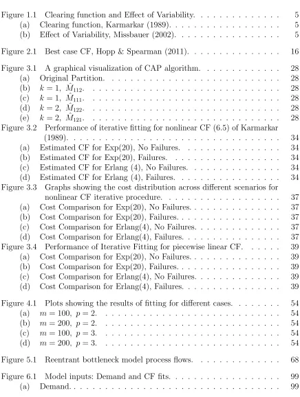
Clearing functions are non-linear functions that describe the expected output of a re-source over a given period as a function of expected workload over that period. Queuing theory provides the theoretical basis for several such functional forms. Several authors (Karmarkar, 1989; Srinivasan et al., 1988; Graves, 1986; Missbauer, 2002; Asmundsson et al., 2009) derived clearing functions from different assumptions about the underlying model of production system under consideration. Despite the differences in functional forms proposed, most CFs have the following properties

Properties

1. CFs are concave, continuous, monotone and non-decreasing functions of workload.

2. As a consequence of the above property, CFs have a diminishing rate of return. i.e, the percentage increase in output is less than the percentage increase in output i.e., the maximum expected output possible in a planning period.

3. limx→+∞f(x) =C where C is the nominal capacity of the resource.

4. The curvature of the CFs decreases with increasing variability of the system as shown in 1.1(b).

1.2 Literature Gap

(17)

Saturating

F ixed Lead T ime

F ixed Capacity

E[W orkload]

E

[

O

utput

]

(a)Clearing function, Karmarkar (1989).

c= 0

c= 0.5

c= 1

E[W orkload]

E

[

O

utput

]

(b)Effect of Variability, Missbauer (2002).

(18)

LP formulation, the underlying non-linear optimization problem has not attracted much attention due most studies focusing on using piecewise linearization of the CF. Although linearization leads to a LP representation of PP-CF, the solution quality with respect to the number of segments have not been explored. By solution quality we mean in particular the variability in the release pattern and other quantities of interest like inventory, work in progress and the realized cost of implementing the plan. It is well known from Hopp & Spearman (2011) that variability in releases has a negative impact on the cycle time of the production system. Practical implementation of the release pattern obtained from the LP models can be very challenging if the releases in the optimal plan fluctuate significantly from one period to another. The fitting procedure for estimating CF parameters has issues such as sampling bias, non-convexity, etc. Further, the proposed non-linear CFs do not extend well to almost deterministic systems, which provide a piecewise linear CF on visual inspection. Either the functional forms are not flexible enough to model to these situations, or the fitting problem is non-convex making it difficult to obtain globally optimal estimates. The estimation of parameters becomes crucial due to the sensitivity of the system performance (profit) to changes in these parameters (Asmundsson et al., 2009; Kacar & Uzsoy, 2015). The least squares estimates are known to be sensitive to outliers and the symmetric penalty for over-estimation and under-estimation does not represent the problem quite well. Asmundsson et al. (2009) showed that a percentile fit can yield better performance than the LSE fit. Motivated by these studies and issues presented above our contribution to literature through this thesis is presented next.

1.3 Contributions

In this dissertation several advancements to PP-CF are presented

(19)

2. In Chapter 4, the problem of fitting the CF and then linearizing it for further use in optimization is addressed by direct piecewise linear fitting to the data. The MILP formulation proposed by Toriello & Vielma (2012) is examined and valid inequalities are added to reduce the solution time. This formulation is effective in fitting CF when the number of observations is small to medium (n≈1000). For larger datasets, the convex adaptive partitioning (CAP) proposed by Hannah & Dunson (2013) is used. Computational experiments show that the proposed piecewise fitting yields better performance.

3. The problem of allocating output to products in the workload ratio is addressed in ACF formulation (Asmundsson et al., 2009) by approximating the non-convex FIFO constraints. A new data driven approach using Mean Value Analysis (MVA) is recently presented by Omar et al. (2017). In Chapter 5, we conduct experiments to help understand the advantages and shortcomings of the data-driven (DD) model in relation to the ACF model.

4. In Chapter 6, a conic reformulation of the PP-CF problem is proposed. The non-linear programming is convex but not differentiable everywhere which prevents the use of conventional calculus based methods for solving the problem. We also provide conic reformulations of several CFs proposed in literature. Conic programming provides an elegant duality theory analogous to LP, which is used to extend the duality analysis to PP-CF. The solution quality and dual prices are more accurate with the proposed reformulation.

1.4 Outline of the Dissertation

(20)

(21)

Chapter 2 Previous Related Work

The use of mathematical programming models for production planning has a long history, dating back to the seminal work of Holt et al. (1955). The problem was formulated as an optimization problem with a quadratic objective function with material flow balance constraints. The unrealistic behavior of conventional LP models such as instantaneous output or workload independent lead-time can be addressed with integration of information from system data in the optimization models. Holt et al. (1955) and Holt et al. (1960) used historical data to estimate the coefficient of the variables in the objective function of the optimization problem.

An important problem in production planning is that of determining the timing and quantity of work releases into the production system to ensure that output matches demand in an optimal or near-optimal manner. This must consider thecycle time, the delay between work being released into the production system and its emergence as finished product. Both queuing theory (Buzacott & Shanthikumar, 1993) and simulation models (Atherton & Atherton, 1995) have demonstrated a nonlinear relation between mean cycle time and mean resource utilization. In general, the cycle time of a job through a production system is a random variable whose distribution depends on the level of resource utilization, among other factors. However, resource utilization is determined by the workload, the amount of work available to a resource in a planning period, which is, in turn, determined by the release decisions made by the planning model. This circularity, where the cycle time depends on release decisions that themselves require knowledge of the cycle times, has been a persistent issue in production planning.

(22)

by far the most common, is to represent cycle times as a workload-independent, exogenous lead time as in the Material Requirements Planning (MRP) procedure (Vollmann et al., 2005) and most linear (LP) and mixed integer (MIP) programming models for production planning (Hackman & Leachman, 1989; Missbauer & Uzsoy, 2011a). This approach yields computationally tractable models, but fails to capture the workload-dependent behavior of cycle times, particularly when resource utilization varies significantly over time. A second approach has been to decompose the problem into two subproblems, one that determines optimal releases for given cycle time estimates and another that estimates the cycle times that will be realized under these releases (Hung & Leachman, 1996; Kim & Kim, 2001; Byrne & Hossain, 2005). The first is usually a LP, while simulation, queuing or regression models can be used for the latter (Hung & Hou, 2001). The algorithm iterates between the two models until convergence is achieved. However, the computational burden of these approaches is high due to their use of a detailed simulation model, and their convergence is not yet well understood (Irdem et al., 2010).

2.1 Clearing Function models

The third approach, which motivates this work, uses nonlinear clearing functions (CFs) that represent the expected output of the resource in a planning period as a function of its planned workload during that period (Missbauer & Uzsoy, 2011a). The CF can be viewed as a metamodel of the queuing system representing the production resource, characterizing its expected output over a range of workload levels. Most of the literature has focused on developing CFs that can be incorporated into tractable mathematical programming models, generally using the total workload of all products at the resource in the planning period as the independent variable. The use of a single independent variable resulted in difficulties representing production systems with multiple products, which are largely, though not completely, resolved by the Allocated Clearing Function model of (Asmundsson et al., 2009) in the absence of lot sizing. A growing body of research has shown that planning models using appropriately parameterized CFs can yield improved production plans over both fixed lead time and iterative multi-model approaches, especially when resource utilization varies over time (Asmundsson et al. 2009; Kacar et al. 2013, 2016).

(23)

1986, Karmarkar, 1989 and Srinivasan et al., 1988. These CFs use a single state variable, either the work in process inventory (WIP)Wt−1 at the resource at the start of periodt, or

the workload Λt, in units of time, available to the resource over the planning period. The

workload Λt denotes the total amount of work, measured in units of time, that becomes

available to the resource in periodt, and is given by Λt= Wt−1+Rt, whereRt denotes the

amount of material released to the resource in period t, again in units of time. Motivated by steady-state queuing models, Karmarkar (1989) suggests the functional form

f(Λt) = min n

Λt,

K1Λt K2+ Λt

o

, Λt≥0 (2.1)

where K1 is set equal to the maximum expected output in a planning period and K2 is a

parameter to be estimated from data. Motivated by results from traffic modeling (Carey & Bowers, 2012), Srinivasan et al. (1988) suggest the form

f(Wt) = K3(1−eK4Wt), Wt≥0 (2.2)

where K3 andK4 denote parameters to be estimated. Missbauer (2002) proposes the form

f(Λt) =

1 2

h

C+k+ Λt− p

C2 _{+ 2}_Ck₊_k2₋₂_C_Λ

t+ 2kΛt+ Λ2t i

(2.3)

where C denotes the length of the planning period andk = 0.5(σ2/τ +τ), where τ andσ denote the mean and variance of the processing time, respectively.

These functional forms are all based on steady state queuing models. However, the CF seeks to represent the behavior of the production resource during a finite planning period, over which the system may not attain steady state. Missbauer (2009; 2011) shows that the shape of the CF for a given value of Λt changes as a function of both Rt and Wt−1, demonstrating that the shape of the CF can vary based on system state. The

incorporation of transient CFs results in complex optimization models that are difficult to solve (Missbauer, 2011), and remains the subject of ongoing research. In this thesis we shall focus on the simpler problem of fitting a single univariate CF to data from a simulation model.

(24)

(6.5) - (6.7) above, and estimate the its parameters from data using linear regression (LR). The CF thus obtained is assumed to represent the expected behavior of the production system at any point in time. However, Asmundsson et al. (2009) found that using LR with a single state variable systematically underestimated the CFs; a heuristic percentile fit yielded much improved results. Kacar & Uzsoy (2015) used simulation optimization to estimate the CF that optimized the performance of the production system, instead of the fit to the data, obtaining substantial improvements in performance over a piecewise linearized LS fit. Kacar et al. (2012; 2013; 2015; 2016) partition the range of data into two segments containing approximately equal numbers of data points, and then use LR to fit linear functions of the workload in each partition. They then add a third segment with slope of zero representing the estimated maximum output of the resource in a period. This approach produces a univariate, piecewise linear CF that is ideal for use in the Allocated Clearing Function formulation (Asmundsson et al., 2009). However, the improved results from simulation optimization (Kacar & Uzsoy, 2015) show that this approach does not always lead to the best possible production plans.

Missbauer’s (2009; 2011) results for transient CFs suggest that a single state variable such as the workload Λt may not be sufficient to describe the behavior of the production

resource accurately. Kacar & Uzsoy (2014) compared a number of linear regression models for fitting workload-based CFs, experimenting with releasesRt, entering WIP Wt−1 and

the same quantities for earlier time periods, as independent variables in their regression models. They found that at high utilization including state variables from earlier periods improves performance, but no single model yields consistently high performance across all experimental conditions. Haeussler & Missbauer (2014) conduct extensive regression analyses using both simulation and empirical data obtained from a manufacturer of optical storage media. They find that incorporating additional independent variables leads to better fits as measured by the adjustedR2, noting substantial differences in results between empirical and simulation data. For bottleneck machines they find that incorporating simple quadratic terms of a single workload variable yields marked improvements in the adjusted R2 _{value. Multidimensional CFs have been proposed for systems with setups}

and lot-sizing decisions (Albey et al., 2014; Kang et al., 2014; Albey et al., 2017), but lead to non-convex optimization models.

(25)

when implemented. In our current state of knowledge, it is not at all apparent that these are the same function.

Clearing functions have been successful in modeling production planning problems with congestion. There is a wide variety of literature on application of clearing functions in tactical production planning. Karmarkar (1989) described a discrete dynamic model using clearing function and also addressed the issues involved in using the clearing function. Karmarkar (1989), Srinivasan et al. (1988), and Missbauer (2002) proposed the functional form of clearing function from queuing theory and traffic flow theory. These functional forms are parameterized with system parameters that are estimated in literature using regression. The data is either obtained from industry or simulation of the factory. The later approach is most widely used due to its ability to model complex system with high accuracy and integration with optimization tools. Later, the model is extended to the multiple product and multi-stage setting by Asmundsson et al. (2009). While over the last two decades, there has been lot of experiments and applications such as dual price estimation under congestion (Kefeli et al., 2011), identifying the bottleneck resource (Kefeli & Uzsoy, 2016), incorporating engineering learning effects (Kim & Uzsoy, 2013; Ziarnetzky & M¨onch, 2016) and capacity expansion (Kim & Uzsoy, 2008) using the underlying linear programming model, not many authors focused on the issue of fitting clearing functions. Asmundsson et al. (2009) proposed a procedure for fitting the clearing function to the data generated from simulation model. The procedure involves generating random demand seeds corresponding to various levels of utilization as release plans to collect WIP and output data from simulation model. A predetermined functional form is fitted to the data using a regression model minimizing the sum of squared errors (SSE). Clearing function estimation using minimizing SSE is unbiased and in systems with high breakdowns the regression underestimates the capacity. This issue is raised by Asmundsson et al. (2009) who propose a biased estimation approach with improved performance. The biased estimate is further considered in Kacar et al. (2012a) where SSE fitting is improved by simulation optimization yielding better performance; again confirming that biased estimate performs better under high utilization.

(26)

of the data used in parameter estimation is different from WIP distribution observed in performance evaluation phase. This can be seen by noting that in a production setting the demand has a distribution whose mean do not vary over the planning period, implying that the mean utilization is constant. Thus the WIP levels should be more concentrated in the range that yields a constant average utilization. The procedures for data collection from simulation used in Asmundsson et al. (2009), Kacar et al. (2012a), and Albey et al. (2014) and the iterative procedures by Hung & Hou (2001) need an initial release plan. This start plan determines the WIP range as well as the data points observed in simulation, establishing a dependence between the release plan and data observed. A similar relationship can be observed in the dependence of production planning models on the initial inventory level. The iteration procedures by Hung & Hou (2001) rely on the convergence of the distribution of the flow time post and pre-estimation. This ensures that the WIP distribution observed in the LP is not different from the WIP distribution in the evaluation phase. This can be regarded as the difference between queuing model prediction and simulation model prediction of flow time or throughput. Selcuk et al. (2008) used utilization as a factor in the design of experiments, implying that fitting procedure was applied to the data generated for a particular utilization which is quite different from the approach proposed by Asmundsson et al. (2009). Thus there is currently no consistency on how to set up the design grid.

(27)

with high variance and less replications at points with low variance. The current procedure for estimating the parameters are in contrary to this variance based allocation approach. Thus there needs to be a systematic way to determine the number of replications of each design point and WIP range. These two factors have significant effect on the parameters estimation.

The estimation by SSE is unbiased; implying it is risk neutral, that may not be the most profitable. In production planning underestimation and overestimation does not have the same risk factor. Losing an order can be more expensive than holding inventory to it. Losing order also affects customer satisfaction the cost of which is more difficult to estimate. Especially in the semi-conductor industry, losing customers could mean losing market share to competitors whereas raw material is relatively cheap compared to underutilized capacity. To counteract this unbalanced risk, the estimation should consider the cost of the underestimation and overestimation. The same phenomenon can be seen in modeling congestion of road networks where arriving late to work can be more expensive then arriving early in flow time estimation. Integrating the cost structure of overestimation and underestimation in to the parameter estimation procedure will underestimate or overestimate the capacity as implied by the trade-off between holding product and losing customers.

(28)

F ixed Capacity

E[W orkload]

E

[

O

utput

]

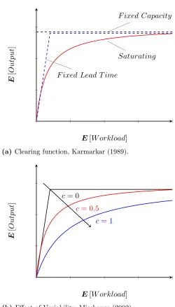
Figure 2.1 Best case CF, Hopp & Spearman (2011).

concave with slope one segment and a constant capacity segment shown in Figure 2.1 (Hopp & Spearman, 2011). Extending the number of segments leads to a problem which is well known in literature as convex piecewise regression. Also, the added advantage being that any concave or convex function can be approximated to arbitrary accuracy by set of affine functions.

(29)

due to the large number of constraints. Mazumder et al. (2015) proposed an efficient computational framework for the QP and used a regularized version of QP to prevent over-fitting. Toriello & Vielma (2012) proposed mixed-integer linear programming (MILP) formulations for parametric (fixed number of segments) and non-parametric fitting, but these do not scale well to large datasets (n≈500).

(30)

Chapter 3 Iterative Refinement Approach

Clearing functions that describe the expected output of a production resource as a function of its expected workload have yielded promising production planning models. However, there is as yet no fully satisfactory approach to estimating clearing functions from data. We identify several issues that arise in estimating clearing functions such as sampling issues, systematic underestimation and model misspecification. We address the model misspecification problem by introducing a generalized functional form, and the sampling issues via iterative refinement of initial parameter estimates. The iterative refinement approach yields improved performance for planning models at higher levels of utilization, and the generalized functional form results in significantly better production plans both alone and when combined with the iterative refinement approach. The IR approach also obtains solutions of similar quality to the much more computationally demanding simulation optimization approaches used in previous work.

3.1 Introduction

The problem of fitting a univariate CF to data obtained from a simulation model appears simple in principle. Given a validated simulation model of the production resource of interest, the principal experimental factor of interest is the workload Λt available to the

resource in each planning period t. An experimental design would then simulate the resource at different levels of Λt, collecting observations Xt of the output obtained in each

period t. The resulting observations (Λt, Xt) would then be used as input to a regression

(31)

CF we seek to estimate, determines the release of work into the production system over time to optimize some objective function. Thus it is impossible to specify the workload in a given planning perioda priori. The ability to control the covariate sampling - the workload levels in each planning period - is essential for variance based sampling or adaptive sampling procedures to obtain parameter estimates with low variance (Fowler et al., 2008). The presence of the planning model also influences the workload samples that can be obtained. Under time-varying demand, a capacitated planning model will tend to distribute workload from periods with high demand to earlier periods with lower demand, again affecting the distribution of workloads likely to be observed. If, in addition, the planning model uses CFs to represent the production resources in the system, the release decisions made by the planning model will depend on the estimated CF used, introducing another source of dependency. Most fitting approaches used in the literature do not take the presence of the planning model into account, ignoring these difficulties and producing biased fits as discussed in Asmundsson et al. (2009).

This chapter explores the problem of fitting CFs to data from simulation models as discussed in chapter 1, taking into account both the presence of the planning model and the dependence between the realized release decisions and the parameter estimates used in the planning model. After reviewing previous work, we identify several difficulties in § 3.3, and suggest a heuristic solution analogous to the policy iteration algorithm used in stochastic optimization in§ 3.5. In §3.6 we present computational results for simple single-stage systems. We conclude the paper with a discussion of our principal findings and directions for future work.

3.2 Previous related work

(32)

models (Missbauer, 2009; Missbauer & Uzsoy, 2011a).

3.3 Issues in fitting clearing functions

In this section we first propose a simple formulation of the problem of fitting a CF to data from a production system, specifying the data to which the fitting procedure will be applied and how the CF is used in the production planning model. For simplicity of exposition we consider a single production resource producing a single product whose behavior can be described as a queuing system, and the functional form (6.5) of Karmarkar (1989); the issues we raise remain valid regardless of the specific functional form we seek to fit. Clearly, if we cannot develop an effective method for fitting CFs for this problem, we cannot hope to make progress for more complex multi-item multi-stage systems. We also assume that we have access to a simulation model of the production system that represents its behavior to a sufficient degree of accuracy. We shall adopt the convention of using bold face to represent a random variable, e.g., X, and normal font, e.g., X to represent a specific realization of that random variable or a deterministic decision variable.

3.3.1 Problem formulation

The effective processing time P of each unit of work (jobs) at the resource, including detractors such as machine failures, quality problems, setups and so on, is a random variable, as is the demand Dt in each periodt. Releases into the system are computed

by a planning model that seeks to determine the amount of material Rt released to the

resource at the start of periodt over a planning horizon ofT periods. In order to focus on the fitting of the CF, we shall assume that at the time the planning model is solved the specific realization of demand to be met over the next T periods is known with certainty. The other decision variables are ˆIt, the amount of finished inventory on hand at the end of

period t; ˆBt, the number of units backordered at the end of period t; ˆWt, the WIP at the

end of periodt; and ˆXt, the output of the resource in periodt. The hats over the decision

variables indicate that these are planned, not realized quantities; the hat is omitted for the Rt to indicate that the releases can be implemented with certainty. Due to the uncertainty

of the effective processing times P, the realized values of all other decision variables are random variablesWt,Xt,Bt, andIt. The fact that Wt is a random variable implies that

(33)

planning model can be written as the following convex optimization problem:

min

T X

t=1

htIˆt+wtWˆt+btBˆt

(3.1)

s.t. ˆ

Wt−1−Xˆt+Rt= ˆWt t= 1, . . . , T (3.2)

ˆ

Xt+ ˆIt−1−Bˆt−1−Iˆt+ ˆBt=Dt t= 1, . . . , T (3.3)

ˆ

Xt−f Wˆt−1+Rt

≤0 t= 1, . . . , T (3.4)

ˆ

Xt,Iˆt, Rt,Wˆt,Bˆt ≥0 t= 1, . . . , T (3.5)

where wt, ht and bt represent the unit WIP holding, inventory holding and backordering

costs, respectively. This captures both the dependency of the planning model on the estimated CF parameters in constraint (3.4), and its basic behavior in redistributing workload across time to account for the limited output capacity of the system. For simplicity we shall assume a static planning model, whose release decisions are not updated on a rolling horizon basis but are implemented as obtained from the planning model for all periods t= 1,· · · , T. Once releases have been determined by the planning model, the expected value of the objective function (3.1) is estimated using multiple replications of the simulation model.

We shall limit ourselves to the situation where the parameters of the CF remain constant for all periods t = 1· · · , T in the planning horizon; allowing time-dependent parameters would not materially alter the fitting problem except by increasing the number of parameters to be estimated. Although the demand is known with certainty at the time the planning model is solved, we seek the planning model of the form (3.1) - (3.5) that yields the lowest expected value of the objective (3.1) over all demand realizationsDt of

the random demand Dt that the system may encounter. The CF we seek represents the

conditional expectation of output in a planning period given a value of the workload Λ. If we denote the set of all random variables representing workload over time byΛ, this expectation is given by

f∗(Λ) = ED,P

h

¯ X|Λ

i

(34)

3.3.2 Control of Covariates

At the time the model is solved, the only parameters known with certainty are the initial WIP and finished goods inventory levels W0 and I0, the cost parameters and the specific

demand realization Dt. The optimal values ˆRt are computed by the planning model and

can be implemented directly. However, the values of ˆXt,Iˆt and ˆWt obtained from the

model (3.1) - (3.5) represent planned, or predicted, values of the realized quantities, which are random variables whose distribution depends, potentially, on the entire history of the production system up to the time they are observed as well as the distribution of the processing times, the dispatching or scheduling procedures used on the shop floor, and other work practices that are abstracted away in the model. Thus the workloads Λt=Rt+Wt−1 that will be observed in the simulation model, and that constitute the

independent variables in the regression model used to estimate the CF parameters, are random variables whose values cannot be directly controlled in an experimental design.

Missbauer, 2011, in his analysis of a CF for a system governed by an M/M/1 queue, demonstrates that the expected output Xt in a future planning periodt depends on both

the initial WIP Wt−1 available at the start of the period and the new releases Rt, and

is a decreasing function of the variability of Wt−1. However, the planning model must

use a deterministic planned value as the argument of its CF in (3.4), replacing a random variable with a deterministic point estimate. We show below that by Jensen’s inequality (Jensen, 1906), this will lead to systematic overestimation of the expected output E[Xt].

3.3.3 Sampling issues

We perform a number of simulation replications g = 1, ..., G that simulate the operation of the production resource over a time horizon of T discrete periods. This yields T G observations Xgt,Λgt

, denoting the observed outputXgtand workload Λgtof the resource

(35)

variables from which the CF is estimated. Incorrect estimates of the CF parameters can cause the planning model to produce release patterns that would not occur with the correct CF (3.6), resulting in observations Xgt,Λgt

that are unlikely to occur with the correct CF.

In most previous research (Asmundsson et al., 2009; Kacar et al., 2016a), CFs were fit using data obtained by simulating the system without considering any planning model, simply setting releases equal to demand in each period to obtain the observations

Xgt,Λgt

. However, ignoring the presence of the planning model in this way is likely to distort the sample of observations obtained, as illustrated in Section 3.6. In periods of high demand, the planning model will not release all of a period’s demand in the period it is needed, since this will cause high resource utilization and long cycle times; instead, it will release some of this material earlier, building finished goods inventory from which future demand can be met. This behavior of the planning model will materially affect the joint distribution of the workload at the production resources in a given planning period and the output in that period, and thus the parameters of the fitted CF. A notable exception is the work of P¨urgstaller & Missbauer, 2012 who first simulate the system with periodic releases equal to demand, without any planning model. These results are then used to estimate average cycle times and load limits at the different workcenters. A second simulation is then conducted using the workload control approach of Hendry & Kingsman, 1991 to control releases such that workloads do not exceed the workcenters’ specified load limits. The data from this second set of simulations, where the releases are controlled based on the capacity of the system, are then used to fit the CF used in their experiments. Thus the data used to fit their CF considers limited capacity, although not through the explicit representation of a planning model as we do in this paper.

3.3.4 Regression issues

The functional forms used in previous work create substantial problems for a regression approach. It is evident that the CF has to satisfy f(∆t) ≤ ∆t, implying that output

(36)

workload, the associated regression problem requires solution of a non-convex optimization problem whose global optimum is difficult to obtain.

3.3.5 Functional forms derived from steady-state queuing

mod-els

Another set of issues arises from the use of functional forms derived from a steady state queuing model, which we shall illustrate using the CF (6.5) of Karmarkar (1989), without the minoperator as discussed above. The second term under the min operator in (6.5) is derived from the steady state M/M/1 queuing model, yielding a regression model of the form

Xt=f(Rt,Wˆt−1) +εt=

K1(Rt+ ˆWt−1)

K2+ (Rt+ ˆWt−1)

+εt, ∀t= 1, ...., T (3.7)

where εt is, ideally, normally distributed with a mean of zero and standard deviation σ. The time independence ofσ assumes the absence of heteroscedasticity, i.e., that the variance σ of the residual error is independent of the workload, which is often not the case. The queuing analysis motivating the functional form makes a different statement, which is that

E[Xt] =f(Rt, E[Wt−1]) =

K1(Rt+E[Wt−1])

K2+ (Rt+E[Wt−1])

(3.8)

Taking the expectation of (3.7) and assuming that the optimal values of the decision variables represent unbiased estimators of the realized quantities - a highly questionable assumption - we obtain

ˆ

Xt=E[Xt] =E

h

f(Rt,Wˆt−1)

i

≤f(Rt, E[Wt−1]) (3.9)

by Jensen’s inequality (Jensen, 1906) and the observation that (6.5) is concave in both Rt and Wt−1. This suggests the distinct possibility that, even under the highly idealized

(37)

output in a planning period. This argument remains valid for any functional form derived from steady-state queuing analysis that relates the expected output to the expected value of some workload-related random variable. This again calls into question the desirability of using functional forms derived from steady-state queuing models, suggesting the need for an alternative approach.

3.4 The min-affine functional form

The bounded and concave structure of the CFs suggests using a concave piecewise linear function, eliminating the need for outer linearization and the need to choose a specific nonlinear functional form. Further, since any concave function can be approximated with amin-affine (minimum of a finite number of affine functions) function, we can directly fit the data with the min-affine form without losing the model’s ability to represent the data. The general min-affine form withk affine segments can be written as

f Λt

= min

c∈ {1,..,k}

αcΛt+βc . (3.10)

A significant advantage of (3.10) is that it can be generalized to multivariate settings as long as the concavity is valid, as is the case when Rt and Wt−1 as covariates because the

output is non-decreasing in Rt and Wt−1 (Missbauer, 2011).

In this chapter we use the min-affine functional form and compare its performance to that of the nonlinear CF (3.7) of Karmarkar (1989). We fit the min-affine using the Convex Adaptive Partitioning (CAP) algorithm proposed by Hannah & Dunson (2013), details of which are briefly summarized in the Appendix together with an illustrative example. We now turn to addressing the sampling issues discussed above.

3.4.1 The Convex Adaptive Partition (CAP) Algorithm

We first introduce some notation required to describe the CAP procedure. Gven the data

{xi, yi}ni=1, let X denote the covariate space of the (of the xi) which is partitioned into

non-intersecting subsets {A1, ...., AK}, Ak ⊆ X ∀k. The observation partition (of the yi)

is defined based on the covariate partition as

(38)

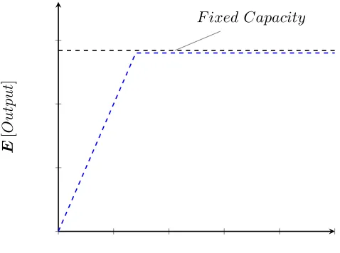
A modelMkis jointly defined by: 1) the covariate partition{A1, ..., AK}of the covariate space, 2) the corresponding observation partition {C1, ..., CK}, and the hyperplanes

{αk, βk}Kk=1 corresponding to these partitions. A knotalrepresents the proportion between

the splits. Starting from an initial partition, the CAP algorithm progressively refines the partition until no subset can be split without creating at least one subset having fewer than the minimal number of observations

nmin = min

n n

Dlogn,2(d+ 1)

o

.

whered is the dimension of the covariate spaceX (1 in the case of a univariate CF) andD

a log scaling factor, which acts to change the base of the log operator. The minimum subset size nmin is chosen to admit O log(n)

subsets to ensure consistency of the estimator (Nobel, 1996) and prevent over-fitting of the data. The algorithm of Hannah & Dunson (2013) can be stated as follows:

Algorithm CAP:

Step 1: Initialize. Set K= 1; define model M1 by placing all observations into a

single observation subset C1 ={1, ..., n};A1 ={xi}ni=1.

Step 2: Split. Refine partition by splitting a subset.

(a) Generate candidate models ˆMkjl by

i. Fixing a subset k,

ii. Fixing a dimension j of the covariate space

iii. Dyadically dividing the data in subset k and dimensions j according to knot al.

This is done for Lknots, all d dimensions and Ksubsets. For example, given a subsetCk, k ∈ {1, ...,K}and dimensionj ∈ {1, ..., d}, let xijkmin = min{xij :i∈ Ck}, andxijkmax = max {xij :i∈Ck}. We define 0< a1 <· · ·< aL<1 be a set

of evenly spaced knots that represent the proportion between xijk_min and xijk max.

(b) Select the candidate model MK+1 that minimizes global mean LSE on the

training set by settingMk ={Mˆjkl: jkl

= argminj,k,l_n1 n P i=1

(39)

with ˆfjkl _x i

= maxi∈{1,..,K}αjkli +β jkl

i xi such that minkkCkk ≥ nmin. Set K=K+ 1.

Step 3: Refit. Use the partitions A0_k = {xi : αk+βkTxi ≥ αj +βjTxi, j 6= k}

induced by the hyperplanes {αk, βk}Kk=1

to generate modelM_K0 . SetMK =MK0 if for every subset C_k0 inM_K0 , kC_k0k ≥nmin.

Step 4: Check stopping conditions. If for every subsetCk inMk,kCkk<2nmin,

stop fitting and proceed to Step 5. Otherwise, go to Step 2.

Step 5: Select model size. Each model Mk creates an estimator,

fk x

= min

j∈{1,..k}αj+β

T j x

(40)

C₁ C₂

(a)Original Partition.

b

112

C₁₁ C₁₂ C₂

(b)k= 1, M112ˆ .

b

111

C₁₁ C₁₂ C₂ C₁₁ C₁₂ C₂

(c) k= 1, M111ˆ .

b₁₂₂ C₁ C₂₁ C₂₂

(d)k= 2, Mˆ122.

b₁₂₁ C₁ C₂₁ C₂₂

(e) k= 2, Mˆ121.

Figure 3.1 A graphical visualization of CAP algorithm.

The CAP procedure described above can be viewed as an alternative to classical least-squares regression that fits the min-affine functional form (3.10) to data. However, this procedure is subject to the same difficulties raised by the presence of the planning model: the inability to control the values of the workload (the independent variable) directly in the experimental design, and the dependency between the observations and the estimated parameters of the CF. The Iterative Refinement procedure addresses these limitations directly, and can be used for any fitting procedure.

To illustrate the operation of the algorithm, consider the data in Figure 3.1 with covariates x={1,2, ...,100}. We start with the optimal split that minimizes global LSE with two partitions given by Figure 3.1 (a). We would like to split the partitions further using knots a1 = 1/3 anda2 = 2/3. Figures 3.1 (b) and (c) are splits of subsetk = 1, with

(41)

b111 = 0.3×55 + 0.7×1 = 17.2 giving the partitions as in Figure 3.1 (c) and fora2 = 2/3,

we get b112 = 38.8 resulting in partition shown in Figure 3.1 (b). Similarly, for subset

k = 2 we have the partitions shown in Figures 3.1 (d) and (e). Since covariate space is univariate we do not have partitions in the dimension. Figures 3.1 (b) - (e) each have 3 partitions, to each of which a linear model is fit. The global LSE is calculated by taking the min-affine form corresponding to the 3 linear segments as the model prediction. The model with minimal SSE among the four given models is selected as specified in Step 2: (b) resulting in a model with 3 partitions which is again partitioned by similar approach

until the stopping criteria are met.

3.5 Iterative Refinement procedure

The Iterative Refinement procedure is applicable to the fitting of any functional form, and starts with an initial estimate of the CF parameters. At each iteration the current estimates of the parameter values are implemented in the planning model, and the system is simulated to obtain observations of workload and output. In our experiments we obtained initial parameter estimates using the most common procedure in the literature to date (Asmundsson et al., 2009; Kacar et al., 2012a), which we shall refer to as Unplanned CF Estimation, since it does not consider any planning model. This procedure can be stated as follows:

Algorithm UCF (Unplanned CF Estimation)

Step 1: Identify a set of target mean utilization levelsρj, j = 1, ..., J that span the

range of utilizations the system is expected to experience under its routine operating conditions

Step 2: For each value of ρj, generate M independent realizations of demand that

yield a mean utilization level of ρj. This yields a total ofJ M independent demand

realizations

Step 3: For each demand realization, set releases in each period equal to demand in that period, i.e., Rt=Dt, and simulate the execution of this release plan forG

(42)

Step 4: Use the J M GT observations obtained in Step 3 to obtain estimates of the CF parameters KU _{= (}_KU

1 , K2U) using the selected fitting procedure.

Different fitting procedures can be used in Step 4 depending on the specific functional form used. In our experiments we use linear regression to fit the nonlinear functional form (6.5), and the CAP procedure of Hannah & Dunson (2013) described in the Appendix to

fit the min-affine functional form (3.10).

The UCF procedure does not take into account the production planning model, effectively ignoring the impact of limited capacity on releases. As a result, the workload levels generated by the simulation will differ substantially from those encountered when the system operates using a capacitated planning model. A capacitated planning model will tend to redistribute workload over time, producing ahead of periods with high demand to reduce workloads in those period while increasing it in earlier periods. Thus the joint probability distribution of the (∆t, Xt) observations may differ substantially from those

that would be obtained with the correct CF. The Iterative Refinement procedure starts with the vector KU _{of parameter estimates obtained by the UCF procedure and refines}

them iteratively by running new simulation replications with the updated releases (re-sampling) and refitting until either no significant change in the parameter estimates is observed or a maximum number of iterations maxIter is reached. The procedure can be stated as follows:

Algorithm IR (Iterative Refinement):

Step 1: Identify a set of target mean utilization levelsρj, j = 1, ..., J that span the

range of utilizations the system is expected to experience under its routine operating conditions

Step 2: For each value of ρj, generate M independent realizations of demand

that yield a mean utilization level of ρj, for a total of J M independent demand

realizations.

Step 3: Set i= 0, Ki ₌ _KU_.

(43)

aug-mented with the following constraints which we have found to improve the fit:

Xt≤Ct ,t = 1, ..., T (3.11)

Xt≤Rt+Wt−1 , t= 1, ..., T. (3.12)

Constraint (3.11) ensures that expected output does not exceed the expected capacity of the system, while (3.12) ensures that the output in any period cannot exceed the planned workload. Note that the original CF (6.5) of Karmarkar (1989) includes both these constraints, but we do not include them in the LS fitting process due to the need for constrained regression to enforce these. Simulate the execution of each release plan forGindependent replications, obtaining a total ofJ M GT observations (Xgt,Λgt).

Step 5:Use theJ M GT observations obtained in Step 3 to obtain revised parameter estimates Ki+1 _{using the selected fitting procedure.}

Step 6: Ifi > maxIter or

0≤ kK

i+1₋_Ki_k kKi_k ≤ε,

stop and return Ki+1. Otherwise set i=i+ 1, go to Step 3.

(44)

However, the proof of convergence of policy iteration to an optimal policy requires that the cost of the updated policy at each iteration is at least as good as that at the previous iteration, which cannot be guaranteed in the IR algorithm because the value function is not directly linked to the policy improvement step (regression). Feasible solutions at a given iteration need not be feasible in the next one; the CFs fitted at successive iterations may cross each other, making a general proof of convergence to an optimal set of CF parameters difficult.

3.6 Computational experiments

Our computational experiments examine the performance of the Iterative Refinement procedure on four simple single-stage single-item production systems whose characteristics are summarized in Table 3.1. All times are given in minutes. External demand follows a binomial distribution with n = 100 and success probability pchosen to yield the desired mean utilization level. Hence demand variability is not constant across all utilization levels. We consider a planning horizon of T = 26 periods, each of length 1440 minutes. Separate, independent data sets are used to fit the CFs and to evaluate their performance. We compare the performance of three different release planning procedures. The first two

Table 3.1 Experimental Design.

Factor Values Levels

Service Time Distribution Exponential (20), Erlang (4) 2

Failure Distribution

None

Time to Failure: Gamma (14400,1) Time to Repair: Gamma (2400,1.5) 2

Mean Utilization Level 0.3, 0.45, 0.75, 0.9 4

Independent Demand Replications 5

Simulation Replications per Release Plan 5

(45)

independent demand realizations for each level of mean utilization; a release schedule is generated for each demand replication, and its execution then simulated for 5 independent replications to estimate the realized costs of each planning procedure. The planning model assumes a unit back-ordering cost of b = 50, a unit WIP holding cost of w= 6, and a finished goods inventory holding cost of h= 5. The values of these cost parameters will affect the releases produced by the planning model, and hence the fitting of the CF in the Iterative Refinement approach.

We present two sets of experiments. The first use the IR procedure to fit the nonlinear CF (3.7) directly. In the second experiment we use the IR procedure with the convex adaptive fitting procedure to fit themin-affine functional form (3.10).

3.7 Results of experiments

In this section, we analyze the numerical results obtained by iterative fitting of functional forms (3.7) and (3.10), to quantify the effects of ineffective sampling and model misspeci-fication on the average cost of the production system. The Friedman test (Conover, 1980) is a non-parametric test used to compare observations repeated on the same subjects, and uses the ranks of the data rather than their actual values to calculate the test statistic without requiring any distributional assumptions on the data. We perform statistical tests under the null hypothesis that all rankings of the different treatments (in this case, the CF fitting procedures) are equally likely at a significance level of p= 0.05. Thus we compute the expected cost obtained using each fitting procedure for each simulation replication of each demand realization, and observe the relative ranking of the fitting procedures. These rankings then form the input to the Friedman test. The IR algorithm converges in about 8 iterations for the cases with no failures, and within 10 iterations for the cases with failures. To ensure consistent comparisons we fixed the number of iterations at 10 for all experiments.

3.7.1 Nonlinear Iterative Refinement (NIR)

(46)

Unplanned CF obtained using the Unplanned Estimation procedure, and the Iterative CF obtained from the Iterative Refinement procedure. A consistent pattern emerges in these figures: Unplanned Estimation yields CFs that overestimate output at low workloads, and significantly underestimate it at higher workloads. In contrast, the Iterative Refinement CF appears to exhibit high accuracy at lower workloads but to overestimate quite drastically at higher workloads. However, this initial impression is misleading, because the planning model restricts the releases to prevent high workloads in the region where the CF is relatively flat, since this increases WIP holding costs without materially affecting output. Hence the planning model will eliminate the workload levels where the CF from Iterative Refinement appears to have very poor accuracy, causing the system to operate in the region where its accuracy is highest.

0 25 50 75 100 125 150 0

20 40 60 80 100

(a)Estimated CF for Exp(20), No Failures.

0 25 50 75 100 125 150 0

20 40 60 80

(b)Estimated CF for Exp(20), Failures.

0 25 50 75 100 125 150 0

20 40 60 80 100

(c) Estimated CF for Erlang (4), No Failures.

0 25 50 75 100 125 150 0

20 40 60 80

(47)

Figures 3.3(a) through 3.3(d) show the expected costs obtained using the Unplanned and Iterative CFs, with the cost of a naive release policy that sets releases equal to demand in each period included as a baseline. In the absence of failures, there is no significant difference in costs at the lower utilization levels ofu = 0.32 andu = 0.45. This is to be expected, since whether the CF is accurately estimated or not the resource has considerable excess capacity. Atu= 0.75, the Unplanned CF yields worse performance than the Naive policy; Iterative Refinement significantly outperforms Unplanned Estimation, but is not quite as good as the Naive policy. At high utilization, however, Iterative Refinement outperforms both its competitors by a wide margin. This behavior is due to the fact that the planning model keeps the system operating in the region where the Iterative Refinement procedure provides the best fitting CF. In the presence of failures, this performance is sustained, although the higher magnitude of the costs makes it less apparent in the figure. The situation is better observed from Table 3.2, which presents the p-values for the Friedman test comparing the average cost obtained using the Iterative and Unplanned CFs. In the absence of failures the difference between the Unplanned and Iterative CFs is statistically significant at p = 0.05 for all utilization levels above 0.30. When failures are present, the improvement from the Iterative CF remains statistically significant for both processing time distributions at u = 0.90, and at u=0.75 for the Exp(20) case. In no case is the average cost from the Unplanned CF better than that obtained using the Iterative CF.

Examining the average backorder and holding cost achieved by the planning models, we see in 3.3(a) that at u= 0.75, the IR algorithm increases the backorder cost from 52 to 68 while reducing the inventory cost from 1742 to 707. In 3.3(c), however, it reduces the holding cost from 6069 to 1293 atu= 0.75, while in 3.3(d) at u= 0.9 backorder costs are reduced from 24521 to 19359 and holding costs from 8020 to 5685. These observations indicate that the planning models using the IR CF are able to trade off backorder and holding costs effectively depending on the utilization level; the cost savings are not being obtained by reducing backlogs alone.

(48)

Case CF. The inclusion of constraints (3.11), on the other hand, brings the planning model into agreement with the Best Case CF at high utilization levels. Since the Naive policy does not use any planning model, its poor performance at high utilization is to be expected. In the absence of failures at u= 0.75, Figure 3.2 shows that the Unplanned CF lies below the Iterative CF, which, in turn, lies below the Best Case CF. This suggests that both fitted CFs underestimate output, resulting in higher backorder costs. In the cases with failures both fitted CFs are quite close to each other and both result in better performance than the Naive policy. These results suggest that a particular functional form may perform well in some regions of the covariate space and poorly in others, and that different functional forms may be appropriate for different regions of the covariate space. The min-affine functional form discussed in the next section explicitly takes this approach by partitioning the covariate space and fitting a different affine function within each.

Table 3.2 Friedman Test (p value) for mean difference comparison for Unplanned and Itera-tive algorithms with nonlinear CF.

Utilization Exp(20) No Failure Exp(20) Failure Erlang(4) No Failure Erlang(4) Failure

0.30 1.0000 1.0000 1.0000 1.0000

0.45 0.0253 0.3173 0.0253 0.3173

0.75 0.0000 0.0093 0.0000 0.8415

(49)

0.3 0.45 0.75 0.9 0 3000 6000 9000 12000 C o s t in $

515 315 315 543 ₂₉₃ ₂₉₂ 673 1837

810 13044

7800

6120 N aive P olicy

U nplanned CF Iterative CF

(a)Cost Comparison for Exp(20), No Failures.

0.3 0.45 0.75 0.9

0 17000 34000 51000 68000 85000 C o s t in $

2659 2863 2863

6730 7142 6993 23679

20980 20632 87486

35894₃₄₀₃₀ N aive P olicy

(b)Cost Comparison for Exp(20), Failures.

0.3 0.45 0.75 0.9

0 2000 4000 6000 8000 C o s t in $ 515

315 315 543 293 292 580 1896

639

8552 8541

3654 N aive P olicy

(c) Cost Comparison for Erlang(4), No Fail-ures.

0.3 0.45 0.75 0.9

0 17000 34000 51000 68000 85000 C o s t in $

2733 2914 2914

6788 7230 6979 24334

21021 20822 86274

38472 32216 N aive P olicy

(d)Cost Comparison for Erlang(4), Failures.

Figure 3.3 Graphs showing the cost distribution across different scenarios for nonlinear CF iterative procedure.

Production Planning with Clearing Functions: Data-driven Approaches and Conic Programming.

Abstract

Dedication

Biography

Acknowledgements

Table of Contents

LIST OF TABLES

LIST OF FIGURES

Chapter 1

Introduction

1.1

Problem Statement and Motivation

1.1.1

Clearing functions

1.2

Literature Gap

1.3

Contributions

1.4

Outline of the Dissertation

Chapter 2

Previous Related Work

2.1

Clearing Function models

Chapter 3

Iterative Refinement Approach

3.1

Introduction

3.2

Previous related work

3.3

Issues in fitting clearing functions

3.3.1

Problem formulation

3.3.2

Control of Covariates

3.3.3

Sampling issues

3.3.4

Regression issues

3.3.5

Functional forms derived from steady-state queuing

mod-els

3.4

The min-affine functional form

3.4.1

The Convex Adaptive Partition (CAP) Algorithm

3.5

Iterative Refinement procedure

Algorithm UCF (Unplanned CF Estimation)

Algorithm IR (Iterative Refinement):

3.6

Computational experiments

3.7

Results of experiments

3.7.1

Nonlinear Iterative Refinement (NIR)

3.7.2

Iterative Fitting of the

min-affine

functional form