Large Universe Subset Predicate Encryption
Based on Static Assumption (without Random
Oracle)
Sanjit Chatterjee and Sayantan Mukherjee
Department of Computer Science and Automation, Indian Institute of Science, Bangalore
{sanjit,sayantanm}@iisc.ac.in
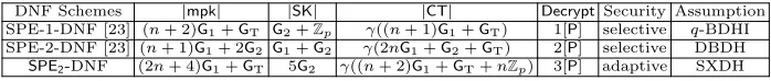
Abstract. In a recent work, Katz et al. (CANS’17) generalized the notion of Broadcast Encryption to define Subset Predicate Encryption (SPE) that emulatessubset containment predicate in the encrypted do-main. They proposed two selectively secure constructions of SPE in the small universe setting. Their first construction is based on a parameter-ized assumption while the second one is based on DBDH. Both achieve constant-size secret key while the ciphertext size depends on the size of the privileged set. They also showed some black-box transformation of SPE to well-known primitives like WIBE and ABE to establish the richness of the SPE structure.
This work investigates the question of large universe realization of SPE scheme based on static assumption in the standard model. We pro-pose two constructions both of which achieve constant-size secret key. First constructionSPE1, instantiated in composite order bilinear groups, achieves constant-size ciphertext and is proven secure in a restricted ver-sion of selective security model under the subgroup deciver-sion assumption (SDP). Our main constructionSPE2 is adaptively secure in the prime order bilinear group under the symmetric external Diffie-Hellman as-sumption (SXDH). Thus SPE2 is the first large universe instantiation of SPE to achieve adaptive security without random oracle. Both of our constructions have efficient decryption function suggesting their practical applicability. Thus primitives like WIBE and ABE resulting through the black-box transformation of our constructions become more practical.
1
Introduction
Katz et al. [23] recently introduced a new primitive called Subset Predicate Encryption (SPE) that allows checking forsubset containment in the encrypted domain. Let IDbe the set of identities. Then, in an SPE, a key SKassociated with a key-index setΩ⊂ IDcan decrypt a ciphertextCTassociated with data-index set Θ⊂ ID ifΩ ⊆Θ. There is an obvious connection between BE and SPE in the sense that both encrypt for a privileged setΘ. However, unlike BE, theKeyGenin SPE takes a set of identitiesΩas input. In terms of functionality, it is trivial to achieve subset containment through multiple membership testing asΩ⊆Θ ⇐⇒ (i∈Ω⇒i∈Θ).
Thus, one may be tempted to use an efficient BE instantiation [9] to construct a small universe (i.e.|ID|=poly(λ) for security parameterλ) SPE. In such an in-stantiation,KeyGenof SPE would simply be a concatenation of output ofKeyGen
of BE for eachx∈Ωi.e.SKΩ= (SKx1, . . . ,SKxk) whereΩ= (x1, . . . , xk). How-ever, such a realization of SPE suffers from an obvious security issue. Given a ciphertext CTΘ, an unprivileged set Ω(having secret key SKΩ forΩ 6⊆Θ) can
easily derive a valid key by strippingSKΩas long asΩ∩Θ6=φ.
In their work, Katz et al. [23] discussed and then ruled out a few generic techniques to construct small universe SPE from Inner-Product Encryption (IPE) [24], Wildcard Based Encryption (WIBE) [1] and Fuzzy Identity-Based Encryption (FIBE) [26] due to the reason of inefficiency. They proposed two dedicated SPE constructions in the small universe setting. Both of their constructions have constant-size secret key while the ciphertext size depends on the cardinality of the privileged set it is intended to. Informally speaking, their first construction utilized theexponent inversion technique [11] and the second one utilized thecommutative blindingtechnique [7]. However, both the construc-tions were proven onlyselectively secure. The security of the first construction is based on a non-static assumption (q-BDHI) whereas the security of the sec-ond construction is based on a static assumption (DBDH). In fact, the secsec-ond construction can be lifted to be selectively secure in the large universe setting, but the proof requires the random oracle assumption.
Given the above results of [23], the main open question in the context of SPE is the following. Can we realize an adaptively secure SPE in the large universe setting under some static assumption without random oracle? In this paper, we answer this question in the affirmative. In addition, we also ask whether one can achieve an SPE with constant-size ciphertext. On this front, this paper reports some partial success through a trade-off in the security model.
restriction in the context of SPE would be that none of the set of identities (here we call key-index set) queried in the key extraction phase should be a subset of the challenge identity set (here we call data-index set). In fact, the security model of SPE introduces two new issues due to aforementioned involved structure of SPE:
– P1: the challenge data-index set might share a few elements with the queried key-index sets.
– P2: the queried key-index sets might have a non-empty intersection among themselves.
We will discuss in details the relevance of P1 and P2 in the context of the security argument of our first construction.
Our first construction (SPE1) structurally is a descendant of IBBE by
Deler-abl´ee [15]. Note that, Delerabl´ee’s IBBE was a constant-size ciphertext construc-tion and was proven selectively secure under aq-type parameterized assumption in the random oracle model. Recently, Gong et al. [18] proposed integration of [15] and D´ej`a Q [30] towards selectively secure IBBE with constant-size ci-phertext under static subgroup decision assumptions in the standard model. Re-call that, the IBBEKeyGen encodes a single identity whereas the SPE KeyGen
encodes a set Ω into a secret key of constant size. However, we show that the
KeyGen of [18] can be tweaked appropriately to generate a constant-size secret key corresponding to a set. This observation leads to our first constructionSPE1,
a constant-size ciphertext SPE in the large universe setting without the random oracle assumption.
The security reduction ofSPE1 uses D´ej`a Q framework just as was done in
[18]. However, we have to address the above mentioned issues (P1 andP2) that stem from more involved structure ofSPE1. Here we report a complete success
against both the issues but in a weaker version of security settings. In some sense, this is the cost we had to bear to construct the first large-universe SPE with constant-size ciphertext. Here we would like to point out that pairing-based construction of an adaptively secure IBBE achieving constant-size secret key and constant-size ciphertext still remains an open problem.
Our main construction (SPE2) achieves adaptive security in the prime order
groups under the SXDH assumption with constant-size secret key. This con-struction resembles the IBBE structure of [25] which extended JR-IBE [22] to achieve an efficient tag-based IBBE construction. We tweak the KeyGen algo-rithm of their IBBE1 [25] to realize adaptive secure SPE in the large universe
setting. Again, the non-triviality lies in the security argument. Precisely, in the security model of IBBE1 [25], for a challenge set Θ∗ = (y1, . . . , yl), the set of identities queried for key extraction should be strictly non-overlapping. In the security argument of (SPE2) however, no such restriction is imposed. In
particu-lar, the query (Ω) adversary makes, may contain some elements that also belong to the challenge setΘ∗.
Here we mention that, our second construction handles both the earlier men-tioned issues completely that too in the adaptive security model. The KeyGen
issue P2 completely. We are thus able to realize the first large universe adap-tively secure SPE without random oracle assumption. Our construction is quite efficient in terms of parameter size, encryption and decryption cost. For exam-ple, the encryption does not require any pairing evaluation while the decryption evaluates only 3 pairings. Only limitation on this construction is obvious: the ciphertext size depends on the size of the privileged set it is intended to.
We conclude with a brief discussion on the effect of the black-box trans-formations due to Katz et al. [23] on our SPE2 constructions. We achieve the
first adaptively secure CP-DNF (CP-ABE with DNF policy) evaluation with a constant-size secret key.
Organization of the Paper. In Section 2 we recall a few definitions and present the notations that will be followed in this paper. In Section 3 we define Subset Predicate Encryption (SPE) and its security model. In Sections 4 and 5, we present two SPE constructions along with their proofs. Section 6 concludes this paper.
2
Preliminaries
Notations. Here we denote [a, b] = {i ∈ N : a ≤i ≤ b} and for any n ∈ N, [n] = [1, n]. The security parameter is denoted by 1λ whereλ∈
N. Bys←- S we denote a uniformly random choicesfromS. ByP(S) we denote the power set of setS. We useA≈Bto denote thatAandBare computationally
indistinguish-able such that for any PPT adversary A, |Pr[A(A)→1]−Pr[A(B)→1]| ≤
where≤neg(λ) forneg(λ) denoting negligible function. We useAdvΠA,M(λ) to denote the advantage adversary Ahas against protocolΠ in security modelM
andAdvAHP(λ) is used to denote the advantage ofAto solve the hard problemHP.
2.1 Bilinear Groups
This paper presents two subset predicate encryption schemes. The first construc-tion is instantiated in the composite order symmetric bilinear groups whereas the second one is instantiated in the prime order asymmetric bilinear groups.
Composite Order Bilinear Pairings. A composite order symmetric bilinear group generatorGsbg, apart from security parameter 1λ takes an additional
pa-rameternand returns (n+ 3)-tuple (p1,· · · , pn,G,GT, e) where bothG,GTare
cyclic groups of orderN = Q
i∈[n]
piwhere allpi are large primes ande:G×G→
GTis an admissible, non-degenerate bilinear pairing [8, 10]. Here,Gpi denotes a subgroup ofGof orderpi. This notation is naturally extended toGpi···pj denoting a subgroup ofGof orderpi× · · · ×pj. By conventiongi···j is an element of
Prime Order Bilinear Pairings. The prime order asymmetric bilinear group generatorGabg, takes security parameter 1λand returns a 5 tuple (p,G1,G2,GT, e)
where all ofG1,G2,GTare cyclic groups of order large primepande:G1×G2→
GTis an admissible, non-degenerate bilinear pairing [17].
2.2 Hardness Assumptions
Composite Order Setting. Let (p1, p2, p3,G,GT, e)← Gsbg(1λ,3) be the
out-put of symmetric bilinear group generator where both G,GT are cyclic groups
of orderN =p1p2p3 wherep1, p2, p3 are large primes. We define two variants of subgroup decision problems [30] as follows:
SD1 : TheSD1problem in groupGis defined as following.
Given g1 ←- Gp1, g3 ←- Gp3, g12 ←- Gp1p2, Z ←- Gp1p2; decide if
Z∈Gp1 orZ ∈Gp1p2.
The advantage of a probabilistic polynomial time algorithmAto solveSD1
is AdvASD1(λ) = |Pr[A(g1, g3, g12, Z) = 1 : Z ∈ Gp1]−Pr[A(g1, g3, g12, Z) =
1 :Z ∈Gp1p2]|where the probability is calculated over the random choice of
g1∈Gp1,g3 ∈Gp3, g12∈Gp1p2,Z ∈Gp1p2 as well as the random bits used
by A. The SD1 assumption holds if for any probabilistic polynomial time algorithmA,AdvASD1(λ)≤neg(λ).
SD2 : TheSD2problem in groupGis defined as following.
Given g1 ←- Gp1, g3 ←- Gp3, g12 ←- Gp1p2, g23 ←- Gp2p3, Z ←- G;
decide ifZ ∈Gp1p3 orZ∈G.
The advantage of a probabilistic polynomial time algorithmAto solveSD2is
AdvASD2(λ) =|Pr[A(g1, g3, g12, g23, Z) = 1 :Z ∈Gp1p3]−Pr[A(g1, g3, g12, g23, Z) =
1 : Z ∈ G]| where the probability is calculated over the random choice of
g1∈ Gp1, g3 ∈Gp3,g12 ∈Gp1p2, g23 ∈Gp2p3, Z ∈ Gas well as the random
bits used byA. TheSD2assumption holds if for any probabilistic polynomial time algorithmA,AdvASD2(λ)≤neg(λ).
Prime Order Setting. Let (p,G1,G2,GT, e)← Gabg(1λ) be the output of
asym-metric bilinear group generator whereG1,G2,GTare cyclic groups of orderpthat
is a large prime.
Symmetric External Diffie-Hellman Assumption (SXDH). The Symmetric Ex-ternal Diffie-Hellman assumption was introduced by Ateniese et al. in [3]. This assumption is defined based on decisional Diffie-Hellman assumption (DDH) on both the source groupsG1 andG2.
DDHG1 : The decisional Diffie-Hellman problem (DDH) in group G1 is defined
as following. Giveng1, g2, gb
1, g
bs
1 , Z=g
s+ˆs
1 ∈G1whereg1 is a generator ofG1,g2
The advantage of a probabilistic polynomial time algorithm A to solve
DDHG1 isAdv
DDHG1
A (λ) =|Pr[A(g1, g2, g1b, g
bs
1 , Z) = 1 :Z =g
s
1]−Pr[A(g1, g2, g1b, g1bs, Z) = 1 :Z=g1s+ˆs,sˆ←-Z∗p]|where the probability is calculated over
the random choice ofg1∈G1, g2∈G2,b, s∈Zp as well as the random bits
used byA. TheDDHG1 assumption holds if for any probabilistic polynomial
time algorithmA,AdvDDHG1
A (λ)≤neg(λ).
DDHG2 : The decisional Diffie-Hellman problem (DDH) in group G2 is defined
as following.
Giveng1, g2, g2c, g
r
2, Z=g
cr+ˆr
2 ∈G2whereg1is a generator ofG1,g2
is a generator ofG2 andc, r←-Zp; decide if ˆr= 0 or ˆr∈Z∗p.
The advantage of a probabilistic polynomial time algorithm A to solve
DDHG2 isAdv
DDHG2
A (λ) =Pr[A(g1, g2, gc2, g
r
2, Z) = 1 :Z =g
cr
2 ]−Pr[A(g1, g2, g2c, g2r, Z) = 1 :Z =g2cr+ˆr,rˆ←-Z∗p] where the probability is calculated over
the random choice ofg1∈G1, g2∈G2,c, r∈Zp as well as the random bits
used byA. TheDDHG2 assumption holds if for any probabilistic polynomial
time algorithmA,AdvDDHG2
A (λ)≤neg(λ).
Note that, in the above description, DDHG1 and DDHG2 are presented in
different manner. The representation of DDHG1 given here is called the 1-Lin
problem which in reality is equivalent to the standard form ofDDHinG1.
3
Subset Predicate Encryption
We next give the definition of Subset Predicate Encryption (SPE) in terms of a predicate encryption [24] and formally model its security requirement.
3.1 Definition
Let ID be the identity space. For a key-index set Ω ∈ X ⊂ P(ID) and a data-index setΘ∈ Y ⊂P(ID), the predicate function for SPE is
Rs(Ω,Θ) = (
1 ifΩ⊆Θ
0 otherwise.
The following description of an SPE scheme is presented here as a Key-Encapsulation Mechanism (KEM) whereC,SKandK denote ciphertext space, secret key space, and encapsulation key space respectively.
– Setup: It takesm∈Nalong with security parameter 1λ. It outputs a master
secret keymskand corresponding public keympk.
– KeyGen: It takesmpk,mskand a key-index setΩ∈ X of sizek≤mas input. It generates a secret keySK∈ SKcorresponding to key-index setΩ.
– Encrypt: It takes mpk, a data-index set Θ∈ Y of size l≤ m as input. It generates the encapsulation keyκ∈K and the ciphertextCT∈ C.
Correctness. For all (mpk,msk) ← Setup(1λ), all key-index set Ω ∈ X, all
SK←KeyGen(msk,Ω), all data-index setΘ∈ Y, all (κ,CT)←Encrypt(mpk,Θ),
Decrypt(mpk,(SK,Ω),(CT,Θ)) = (
κ ifRs(Ω,Θ) = 1
⊥ otherwise .
Remark 1. TheSetupalgorithms takes an additional parametermalong with the security parameterλ. This is because, both our constructions are large universe constructions. The cardinality of the sets processed in ciphertext generation and key generation in both of our constructions will be upper bounded bymlike any other available standard model large universe construction [5, 25].
3.2 Security Definition
Adaptive CPA-Security of SPE. TheIND-ID-CPAsecurity game of SPE is defined between challenger Cand adversaryAas following:
– Setup: The challenger C gives mpk to the adversary A and keeps msk as secret.
– Query Phase-I: Given a key-index setΩ,C returnsSK←KeyGen(msk,Ω).
– Challenge: A provides challenge data-index Θ∗ (such that Rs(Ω,Θ∗) = 0 for all previous key queries).C then generates (κ0,CT)←Encrypt(mpk,Θ∗)
and choosesκ1←-K. It returns (CT, κb) to adversary forb←-{0,1}.
– Query Phase-II: Given a key-index Ωsuch that Rs(Ω,Θ∗) = 0, C returns
SK←KeyGen(msk,Ω).
– Guess: FinallyAoutputs its guessb0∈ {0,1}and wins ifb=b0.
For any adversaryA,
Advind-id-cpaA,SPE (λ) =|Pr[b=b0]−1/2|.
We saySPEisIND-ID-CPAsecure if for any PPT adversaryA,Advind-id-cpaA,SPE (λ)≤ neg(λ). If there is anInitphase before theSetupwhere the adversaryAcommits to the challenge data-index setΘ∗, we call such model selectiveIND-ID-CPAor
IND-sID-CPAsecurity model.
4
SPE
1: Realizing Constant Size Ciphertext
We present the first SPE construction having size secret key and constant-size ciphertext in the composite order pairing setting.
4.1 Construction
– Setup(1λ, m) : The symmetric bilinear group generator outputs (p
1, p2, p3,
G,GT, e) ← Gsbg(1λ,3) where both G,GT are cyclic groups of order N = p1p2p3. Then pickα, β←- N, generatorsg1, u←-Gp1 andg3←-Gp3. Choose
R3,i ←- Gp3 for all i ∈ [m]. Define the msk = (α, β, u, g3) and the public
parameter is
mpk= (g1, g
β
1,
Gi=gα
i
1 , Ui =uα
i
·R3,i
i∈[m]
, e(g1, u)β,H)
whereH:GT→K is a universal hash function for encapsulation key space
K ={0,1}n wheren=poly(λ).
– KeyGen(msk,Ω) : Given a key-index setΩ, such that |Ω|= k≤ m; define the polynomial PΩ(z) = Q
x∈Ω
(z+x) = d0+d1z+d2z2+. . .+dkzk, pick
Y3←-Gp3 and define secret key as
SKΩ=u
β PΩ(α) ·Y
3=u
β Q
x∈Ω
(α+x)
·Y3.
– Encrypt(mpk,Θ) : Given a data-index set Θ, such that |Θ| = l≤ m; the polynomialPΘ(z) = Q
y∈Θ
(z+y) =c0+c1z+c2z2+. . .+clzl. Chooses←-Zp
and computeκandCTΘ= (C0,C1) such that
κ=H(e(g1, u)sβ),C0=gsβ1 ,C1=g
sPΘ(α)
1 =
g
c0
1
Y
i∈[l] Gci
i
s
.
– Decrypt((SKΩ,Ω),(CTΘ,Θ)): AsΩ⊆Θ, computePΘ\Ω(α) = Q
w∈Θ\Ω
(α+w)
= a0+a1α+a2α2+. . . +a
tαt where t = |Θ\Ω|. Then compute κ =
H((B/A)1/a0) where
A=e(C0,Y
i∈[t] Uai
i ), B=e(C1,SKΩ).
Correctness. Notice that, due to orthogonality property,
A=e(C0,
Y
i∈[t] Uai
i ) =e(g sβ
1 , u
PΘ\Ω(α)−a0 Y
i∈[t] Rai
3,i) =e(g1, u)sβ(PΘ\Ω(α)−a0),
B=e(C1,SKΩ) =e(g
sPΘ(α)
1 , u
β
PΩ(α) ·Y3) =e(g1, u)sβPΘ\Ω(α).
Then,B/A=e(g1, u)sβa0,H((B/A)1/a0) =H(e(g1, u)sβ) =κ.
4.2 Security
Recall that SPE1has its root in the Gong et al. [18] modification of the IBBE
to prove the security ofSPE1in the standard model. However, the D´ej`a Q based
argument requires further restriction on the adversary in terms of the key ex-traction queries and we elaborate on this point first.
Recall that, in case of SPE, the adversary A makes key extraction queries on sets. Thus, unlike IBBE, the same identity can be present in more than one distinct key extraction queries. SupposeAmakes key extraction queries on
Ω0={x1,x2},Ω00={x2,x3}andΩ000={x1,x3}wherex1,x2,x3∈ ID. Note that,
the corresponding secret keys in SPE1areSKΩ0 =u
1
(α+x1 )(α+x2 ) · X3
,1,SKΩ00=
u(α+x2 )(1α+x3 ) · X3,2andSKΩ000=u
1
(α+x1 )(α+x3 ) · X3,3. Then, forΩ={x1,x2,x3},
SKΩ=u
1
(α+x1 )(α+x2 )(α+x3 ) =
SKΩ0 SKΩ00
(x3−x1)−1
=
SKΩ0 SKΩ000
(x3−x2)−1
(1)
Precisely, given any two elements from the set{SKΩ0,SKΩ00,SKΩ000}, an adversary
can easily compute SKΩ. Collusion of this sort has already been studied in the
literature and goes by the nameAggregate[16].
If the above-mentioned query sequence{Ω0,Ω00,Ω000} (which results in
cor-responding secret key sequence {SKΩ0,SKΩ00,SKΩ000}) is allowed in the security
game, both the sets{SKΩ0,SKΩ00} and{SKΩ0,SKΩ000} can be combined to make
the same SKΩ. Such a dependency relation also sinks into corresponding
semi-functional components making the D´ej`a Q-based proof fail since it required the semi-functional secret key components to be independent. We call such a query sequence as claw. Allowing claws in the key extraction queries thus lead to a technical problem for the D´ej`a Q-based security argument. This will become clear in the context of our proof ofSPE1 and is discussed further in Footnote 1.
The easiest workaround to avoid suchclaw would be to ensure that no two queries have any element in common i.e.Ωi∩Ωj=φfor all distincti, j∈[q]. In
IND-s∗ID-CPAsecurity model, we put a much weaker restriction on the adversary who is allowed to make key queries only on thecover-freesets. LikeIND-sID-CPA
security model, the challenge data-index set Θ∗ here is committed before the
Setup phase. But the security model restricts the adversary in terms of the queries it can make for key extraction to avoidclaws. Precisely, the adversary in this security model, is allowed to make key extraction queries on the key-index sets (Ω1,Ω2, . . . ,Ωq) adaptively with the restrictionΩi\(Sj∈[q]\{i}Ωj)6=φ. We
say SPEis selective* CPA-secure (IND-s∗ID-CPA) if, for any PPT adversaryA
that gives out the challenge data-index set Θ∗ during Initand the queries it make following above restriction,Advind-sA,SPE∗id-cpa(λ)≤neg(λ).
Here we mention that we do not see any ready vulnerability in our construc-tion due toAggregate(or any other way for that matter). This is because, given the secret keys corresponding toΩi and Ωj, theAggregate computes secret key
forbiggersetΩ(preciselyΩ=Ωi∪Ωj for distinctΩi,Ωj). Now, for a challenge
data-index set Θ∗, the natural restriction ensures Ωi,Ωj 6⊂ Θ∗ and therefore
Ω6⊂Θ∗. Although the existence ofAggregatefunction allowsAto compute the corresponding secret keySKΩ, our security argument establishes that it does not
We reiterate that we do not put any restriction on the relation between the chal-lenge data-index setΘ∗and the queried key-index setsΩapart from the natural restriction Ω 6⊆ Θ∗. The IND-s∗ID-CPA model in this respect behaves exactly same as the IND-sID-CPA model. The restriction imposed in selective*-model is sort of a proof artifact that is inherited in the context of SPE1 from earlier
D´ej`a Q based proofs [18, 30]. The question of arguing security ofSPE1or similar
scheme without the above restriction remains an interesting open problem.
4.2.1 Formal Proof of Security
Theorem 1. For any adversaryAof SPE constructionSPE1in theIND-s∗ID-CPA
model that makes at most q many secret key queries, there exist adversary B1,
B2 such that
Advind-sA,SPE∗id-cpa
1 (λ)≤2·Adv
SD1
B1 (λ) + (m+q+ 2)·Adv
SD2 B2 (λ)
+((m+q)(mp+q+1)+1)
2 + 2
−λ.
Proof. The proof is established via a hybrid argument. The idea is to modify each game only a small amount that allows the solver Bto model the interme-diate games properly. The hybrid argument is based on Wee’s [29] porting of D´ej`a Q framework introduced by Chase and Meiklejohn [12]. In the first game
Game0, both the challenge ciphertext and secret keys are normal. Game1
dif-fers from Game0 as we introduce some simplifying natural restrictions. Game2
reformulates the challenge ciphertext to a different representation that will be useful in later games. InGame3, we replace the challenge ciphertext component
C0 with a random Gp1 element. Then, inGame4, we introduce semi-functional
component in the challenge ciphertext. We next define a sub-sequence of games (Game5,1,0,Game5,1,1,Game5,2,0,Game5,2,1, . . . ,Game5,m+q+1,0,Game5,m+q+1,1)
to introduce entropy into the semi-functional components of secret key and few related public parameters. Note that till this point, we mostly have followed the proof of [18]. Now, the above sub-sequence of games effectively introduces enough entropy in the semi-functional component such that we can replace it with pure random choice inGame6. This game, in particular, uses the property
that key-queries are done on cover-free sets only. Finally, in Game7, we show
that semi-functional components as a whole supply enough entropy to hide the encapsulation keyκ.
Let the adversaryAmake challenge query onΘ∗andqmany key extraction
queries on the sets (Ω1,Ω2, . . . ,Ωq) whereΩi6⊆Θ∗ for alli∈[q]. Let us denote
Θ∗ = {y1, y2, . . . , yl} and Ωi = {xi,1, . . . , xi,ki} for all i ∈ [q]. Then we define sets Ci0 =Θ∗\Ωi and Ci =Ωi\Θ∗ for alli ∈[q] and denote their cardinality
by`0i and `i respectively. The set Mi,j =Ωi\Ωj is the set of identities that is
queried inithquery but not injthquery for alli, j∈[q] andi6=j. Let us denote
Xibe the event thatAhas won the gameGamei.
Game0. This is same as the real game.
– For all z ∈ (Θ∗∪S
i∈[q]Ωi), (α+z) is not divisible by p1. Otherwise,
B can easily solve the subgroup decision problem SD1 by computing
gcd((α+z), N).
– For all i, j ∈ [q] and i 6=j, for all x, x0 ∈ Mi,j, if x6=x0 modN then
x 6= x0 modp2. Otherwise, B can easily solve the subgroup decision problemSD2by computinggcd((x−x0), N).
Therefore,|Pr[X1]−Pr[X0]| ≤AdvSD1B (λ) +AdvSD2B (λ).
Game2. We perform a conceptual change to Game1 here. Given the challenge
data-index setΘ∗={y1, . . . , yl}, pickα,β, u˜ ←-Z2N×Gp1. Define polynomial
PΘ∗(z) = Q
y∈Θ∗
(z+y) and set β = ˜β·PΘ∗(α) modN. In mpk, this affects
only gβ1. Rest of the public parameters in mpk are defined the same as in
Game1. The secret keys corresponding to Ωi is SKΩi = u
˜
β·PΘ∗(α)
PΩi(α) ·Y3 for
i ∈ [q]. The encapsulation key and challenge ciphertext are (κ,CT) where
CT= (C0,C1,C2) such that
κ=H(e(C0, U0)),C0=g
sβP˜ Θ∗(α)
1 ,C1=g
sPΘ∗(α)
1 =C
1/β˜
0 ,
whereU0=u·R3 forR3 ←-Gp3. Note that, the replacementβ = ˜β·PΘ∗(α)
modN doesn’t change the ciphertext distribution as ˜β is uniformly random andPΘ∗(α)6= 0 modp1. Therefore,Pr[X2] =Pr[X1].
Game3. Another conceptual change toGame2 is performed here. ChooseC0←
-Gp1. The rest of the ciphertext is defined the same as inGame2. As bothκ
andC1 are functions of C0, namely κ=H(e(C0, U0)) and C1 =C 1/β˜
0 , such
a replacement doesn’t change the distribution of the challenge ciphertext or the challenge encapsulation key. Therefore,Pr[X3] =Pr[X2].
Game4. Here the subgroup decision assumptionSD1is used to choose C0 from
the group Gp1p2 uniformly at random. Other ciphertext components and
secret keys are generated similar toGame3. Therefore, |Pr[X4]−Pr[X3]| ≤
AdvSD1B (λ). We provide an informal argument here. Given the problem in-stance SD1, B chooses α,β˜ ←- ZN. This allows B to compute all of mpk
similar toGame3. AsBholds bothαand ˜β, it can answer any key extraction
query. In the challenge phase, it uses the targetT of SD1problem instance to simulate C0. If T was from Gp1, C0 is normal whereas if T was from
Gp1p2, thenC0 is semi-functional. SinceC0determines the challenge
cipher-text completely, the distribution from whichT was chosen determines if the challenge ciphertext is normal or semi-functional.
Game5. At this point, we change all the secret keys{SKΩi}i∈[q] and the public
parameters {Ui}i∈[m] to semi-functional. At the same time U0 is also
con-verted into semi-functional. This is done via intermediate games{Game5,k,0,
Game5,k,1}k∈[m+q+1]. Informally speaking, this sub-sequence of games inject
semi-functional component to all of secret keys{SKΩi}i∈[q] and parameters
{Ui}i∈[0,m] multiple times. This is done by repeating the following steps
(i) first addgαmodp2
2 in allSKΩi and allUi forα∈ZN fixed duringSetup, (ii) then replacegαmodp2
2 withg
αk modp2
2 whereαk is a freshly chosen
ran-domness. Here we follow the approach of Wee [30] which lets us argue that all semi-functional components in{SKΩi}i∈[q] and{Ui}i∈[0,m]are random to
adversary (inGame6).
– InGame5,k,0, the parameters{Ui}i∈[0,m] and the secret keys{SKΩi}i∈[q]
are defined as following:
Ui=uα
i
· g2rαi ·g
P
j∈[k−1]rjαij
2 R
0 3,i
SKΩi =u
˜
β·PΘ∗(α)
PΩ
i(α) · g
r·β˜·PΘ∗(α)
PΩi(α)
2 ·g
P
j∈[k−1]
rj·β˜·PΘ∗(αj)
PΩi(αj)
2 Y
0 3
(2)
(3)
Informally speaking, this game “adds” the boxed parts to {Ui}i∈[0,m]
and {SKΩi}i∈[q] of Game5,k−1,1 where r is a uniformly random choice
fromZN. Note that,Bdoes not have explicit access tog2 and simulates
this using the “target” element ofSD2problem instance. We then claim in Lemma 1 that such a modification is invisible to any probabilistic polynomial time adversaryAunder the hardness assumptionSD2.
– InGame5,k,1, as mentioned earlier, we replaceg
αmodp2
2 withg
αkmodp2
2
for a fresh randomnessαk ∈ZN. The change on the parameters{Ui}i∈[0,m]
and the secret key{SKΩi}i∈[q]distributions are shown in the boxed part
below. It is easy to see that we can rewrite Ui and SKΩi in a simpler manner as presented in Equations (4) and (5).
Ui =uα
i
· grkαik
2 ·g
P
j∈[k−1]rjαij
2 R
0 3,i
=uαi·g
P
j∈[k]rjαij
2 R
0 3,i.
SKΩi =u
˜
β·PΘ∗(α)
PΩi(α) · g
rk·β˜·PΘ∗(αk)
PΩ i(αk)
2 ·g
P
j∈[k−1]
rj·β˜·PΘ∗(αj)
PΩ i(αj)
2 Y30
=u
˜
β·PΘ∗(α)
PΩ i(α) ·g
P
j∈[k]
rj·β˜·PΘ∗(αj)
PΩ i(αj)
2 Y
0 3
(4)
(5)
Here we claim that|Pr[X5,k,0]−Pr[X5,k,1]|= 0. First note that, at the
end ofGame4, CT ∗
and κare independent ofα modp2. Moreover, due
toChinese Remainder Theorem, the public parametersg1β,(Gi)i∈[m] are
also independent of α mod p2. Thus, α mod p2 is only present in the
parameters{Ui}i∈[0,m]and in the secret keys{SKΩi}i∈[q]. As a result, the
replacement of α modp2 using αk mod p2 is information-theoretically
hidden to the adversary for freshly chosen uniformly randomαk ∈ZN.
Moreover, r mod p2 is involved only in {Ui}i∈[0,m] and in {SKΩi}i∈[q]
and can be replaced with uniformly random choice rk ∈ ZN trivially.
Here, we denote Game4 by Game5,0,1 and Game5 by Game5,m+q+1,1 to get
a sub-sequence of games that injected requied amount of entropy to all the secret keys and related parameters. The changes that happened be-tween Game4 and Game5 are summed up in Equations (6) and (7) where r1, . . . , rm+q+1, α1, . . . , αm+q+1←-ZN.
uαi·R3,i→uα
i
·g
P
j∈[m+q+1]rjαij
2 ·R03,i
u
˜
β·PΘ∗(α)
PΩi(α) ·Y
3→u
˜
β·PΘ∗(α)
PΩi(α) ·g
P
j∈[m+q+1]
rj·β˜·PΘ∗(αj)
PΩ i(αj)
2 ·Y30
(6)
(7)
Thus, we have|Pr[X5]−Pr[X4]| ≤ P
k∈[m+q+1]
|Pr[X5,k−1,1]−Pr[X5,k,0]|
≤(m+q+ 1)·AdvSD2B (λ).
Game6. Our aim in this game is to show that semi-functional component ofU0is
independent of semi-functional components of (Ui)i∈[m] and (SKΩi)i∈[q]. To
this end, we first replace all semi-functional components of (Ui)i∈[0,m] and
(SKΩi)i∈[q] by freshly chosen uniformly random values and then show that
such a replacement is possible without adversary noticing the change. Thus, we replace theGp2 components of (Ui)i∈[0,m] and (SKΩi)i∈[q] of
Equa-tions (6) and (7) with gz0
2 , g
z1
2 , . . . , g
zm+q
2 respectively for randomly chosen
elementsz0, z1, . . . , zm+q ←-ZN. Precisely, for alli∈[0, m] and for allj∈[q]
we rewrite the Equations (6) and (7) as follows.
Ui=uα
i
·gzi
2 ·R3ˆ ,i, SKΩj =u
˜
β·PΘ∗(α)
PΩ
i(α) ·gzm+j
2 X3ˆ ,j.
This change betweenGame5andGame6can be represented as a linear system
z=Arin Equation (8). In Lemma 2, we show that except with negligible probability, A is a non-singular matrix.1 This ensures z to be a random vector in the span ofA and thus the above modification is invisible to the adversary.
1
This is where the restriction imposed on Ain theIND-s∗ID-CPAsecurity model is useful. As otherwise any clawed query sequence would trivially make A singular. Let us revisit the toy query sequence{SKΩ0,SKΩ00,SKΩ000}that resulted in claw. Let A[m+ 1 +a] encodes Ω0,A[m+ 1 +b] encodesΩ00 andA[m+ 1 +c] encodesΩ000 for some a, b, c ∈ [q]. Then, the following linear combinations A[m+1+(xb]−A[m+1+a]
1−x3)−1
and A[m+1+(xc]−A[m+1+a]
2−x3)−1 makes the rowsA[m+ 1 +b] andA[m+ 1 +c] identical
thereby making A singular. This is where the P2 issue affects our D´ej`a Q based proof argument. The issue P1, on the other hands, does not create any problem in
our proof as PΘ∗(z) PΩi(z) =
Q yj∈Θ∗
(z+yj) Q xj∈Ωi
(z+xj) cancels outPΩi∩Θ
z0 z1 .. . zm
zm+1
.. .
zm+q
=
1 1 · · · 1
α1 α2 · · · αm+q+1 α21 α22 · · · α2m+q+1
..
. ... . .. ...
αm1 αm2 · · · αmm+q+1 ˜
β·PΘ∗(α1)
PΩ1(α1)
˜
β·PΘ∗(α2)
PΩ1(α2) · · ·
˜
β·PΘ∗(αm+q+1)
PΩ1(αm+q+1)
˜
β·PΘ∗(α1)
PΩ2(α1)
˜
β·PΘ∗(α2)
PΩ2(α2) · · ·
˜
β·PΘ∗(αm+q+1)
PΩ2(αm+q+1)
..
. ... . .. ...
˜
β·PΘ∗(α1)
PΩq(α1)
˜
β·PΘ∗(α2)
PΩq(α2) · · ·
˜
β·PΘ∗(αm+q+1)
PΩq(αm+q+1)
· r1 r2 .. .
rm+q+1
. (8)
As a result, we get that|Pr[X6]−Pr[X5]| ≤(m+q)(m+q+ 1)/p2.
Game7. Now we replaceκ0=H(e(C0, U0)) by a uniform random choice fromK.
The reason behind this isU0now isu·g2z0·R3. As we saw in the last game,z0is
a uniformly random quantity independent of all (zi)i∈[q+m]. Thuse(C0, U0) = e(C0, u)·e(C0, g2z0) has logp2 bits of min-entropy due to z0 modp2. Due
to left-over hash lemma [20], κ0 = H(e(C0, U0)) is at most 2−λ distance
from the uniform distribution onK provided Gp2 component in C0 is not
1. The probability that the Gp2 component of C0 is 1 is 1/p2. Therefore
|Pr[X7]−Pr[X6]| ≤ 1/p2+ 2−λ. κ0 now is a random choice and it hides b
completely i.e.Pr[X7] = 1/2.
This completes the proof of Theorem 1 assuming Lemmas 1 to 3 holds.
Lemma 1. There exists PPT adversaryB such that,|Pr[X5,k−1,1]−Pr[X5,k,0]|
≤AdvSD2B (λ).
Proof. The solverB is given the problem instanceD= (g1, g3, g12, g23) and the targetT.
Setup. The adversaryA sends the challenger target setΘ∗.B choosesα,β˜←
-Z2N to generate the public parameters g β
1,(Gi)i∈[m] efficiently where β =
˜
β·PΘ∗(α) mod N, Gi = gα
i
1 . It then chooses {rˆj, αj}j∈[k−1] ←- ZN. The
public parameters (Ui)i∈[m] are generated as follows along withU0 which is
used to computee(g1, u)β=e(g1, U0)β. ForR30,i←-Gp3,
Ui=Tα
i
g
P
j∈[k−1]rˆjαij
23 R
0 3,i.
Bthen outputs public parameter
mpk= (g1, g
β
1,(Gi, Ui)i∈[m], e(g1, U0)β,H),
Phase-I Queries. On a secret key query onΩi, BchoosesY30←-Gp3 and sets
SKΩi =T
˜
β·PΘ∗(α)
PΩi(α) ·g
P
j∈[k−1] ˆ
rj·β˜·PΘ∗(αj)
PΩ i(αj)
23 Y30.
Challenge. B here computes κ0 and CTΘ∗ = (C0,C1) where C0 = g12, C1 = C10/β˜andκ0=H(e(C0, U0)).Bchoosesκ1←-K and outputs (κb,C0,C1) for
b←-{0,1}.
Phase-II Queries. Same as Phase-I queries.
Guess. Boutputs 1 ifA’s guessb0 is same asB’s choice b.
If T ∈Gp1p3, then the game distribution is same as Game5,k−1,1. On the other
hand, if T ∈ G, then the game distribution is same as Game5,k,0 (see
Equa-tions (4) and (5)).
Lemma 2. The matrixAin Equation(8)is non-singular except with probability (m+q)(m+q+ 1)/p2.
Proof. We rephrase the matrixA from Equation (8) as A=
B P
where B∈
Z(pm2+1)×(m+q+1)denotes the first (m+1) rows ofAandP∈Z
q×(m+q+1)
p2 denotes
the lastqrows ofA. Each entry ofBandPare respectively evaluation of follow-ing polynomials with the indeterminant z taking values (α1, α2,· · ·, αm+q+1).
Therefore for anyl∈[m+q+ 1], each [i,l]thentry ofBandPare respectively:
B[i,l] =zi fori∈[0, m],
P[i,l] = ˜
β·PΘ∗(z)
PΩi(z) fori∈[q].
(9)
We simplify the P[i,l] entry next for arbitrary i ∈ SA, l∈ [m+q+ 1].
By natural restriction, for all queries, Ωi 6⊂ Θ∗. Therefore, the polynomial
PΩi(z)6 |PΘ∗(z) for alli∈SAwherezis the indeterminant. Notice that,PΘ∗(z) =
Q
j∈[l]
(z+yj) andPΩi(z) = Q
j∈[ki]
(z+xj) are splitting polynomials. Then, the
ra-tional function
R= PΘ∗(z)
PΩi(z) =
Q
yj∈Θ∗
(z+yj)
Q
xj∈Ωi
(z+xj)
= Q
yj∈Ci0
(z+yj)
Q
xj∈Ci
(z+xj)
=A·B (10)
where A= Q
yj∈Ci0
(z+yj) =PC0
i(z) and B=
1
Q xj∈Ci
(z+xj). It is easy to see that,
B can be rewritten as Q 1 xj∈Ci
(z+xj) = P
xj∈Ci
1
Q xk∈Ci
j6=k
(xk−xj) ·
1
z+xj [21]. In other
words,B= P
xj∈Ci
Rj,i · z+1x
computed from the setCi. The rational fractionRfrom Equation (10) therefore
is
R= X
xj∈Ci
Rj,i·
PC0
i(z)
z+xj
. (11)
For anyi∈SAand l∈[m+q+ 1],
P[i,l] = ˜β· P
xj∈Ci
Rj,i· PC0
i(z)
z+xj (from Equation (9) and Equation (11)) = ˜β· P
xj∈Ci
Rj,i
KC0
i,xj(z) +
tj
z+xj
(tj is scalar)
= P
xj∈Ci
˜
Rj,iKC0
i,xj(z) +
R0j,i z+xj
( ˜Rj,i= ˜β·Rj,i,R0j,i= ˜β·Rj,i·tj are scalars)
= P
xj∈Ci P
k∈[0,`0i]
˜
Rj,i·b j,i k z
k+ R0j,i
z+xj !
(KC0
i,xj(z) = P
k∈[0,`0i]
bj,ik zk is polynomial expansion)
= P
xj∈Ci P
k∈[0,`0i]
˜
R0j,i,kzk+ R
0
j,i
z+xj !
( ˜R0j,i,k= ˜Rj,i·b j,i
k is scalar).
= P
k∈[0,`0i]
ˆ ˜
R0j,i,kzk+ P
xj∈Ci
R0j,i
z+xj ( ˆ ˜
R0j,i,k= P
xj∈Ci ˜
R0j,i,kis scalar).
We rewrite Equation (9) as, for any l∈[m+q+ 1],
B[i,l] =zi fori∈[0, m],
P[i,l] = X
k∈[0,`0i]
ˆ ˜
Rj,i,k0 zk+ X
xj∈Ci
R0j,i
z+xj
fori∈[q]. (12)
Notice that, in Equation (12), each Rˆ˜0j,i,kzk in P[i,l] is in the linear span of
{B[i,l]}j∈[0,m] as `0i ≤ l≤ m. Therefore, elementary row operations remove
such dependency to define a new matrix A0 =
B P0
such that A and A0 are similar matrices (i.e. |det(A)| = |det(A0)|) where for any l∈ [m+q+ 1], z
takes value from the set {α1, . . . , αm+q+1} and each [i,l]th entry of B and P0
are respectively
B[i,l] =zi fori∈[0, m],
P0[i,l] = X
xj∈Ci
R0j,i
z+xj
fori∈[q]. (13)
To complete this proof, it is now sufficient to show the following claim holds.
Claim. The matrixA0 =
B P0
To prove thatA0 as defined above is non-singular, we start from the claim that the matrixD(in Equation (14)) is non-singular if allxj6=xt fort, j ∈[Q]
for t6=j and allγi 6=γk for i, k∈[m+Q+ 1] fori6=k. The non-singularity
ofD was proved in [18, Lemma 3] whereQwas the number of key-queries (i.e.
distinctxj). We here setQto be cardinality of S i∈SA
Ωi
!
i.e. total number of distinctxj that is queried as a part of some key queryΩi.
D=
1 1 · · · 1
γ1 γ2 · · · γm+Q+1 γ2
1 γ22 · · · γm2+Q+1
..
. ... . .. ...
γm
1 γ2m · · · γmm+Q+1 1
γ1+x1
1
γ2+x1 · · ·
1
γm+Q+1+x1
1
γ1+x2
1
γ2+x2 · · ·
1
γm+Q+1+x2
..
. ... . .. ...
1
γ1+xQ
1
γ2+xQ · · ·
1
γm+Q+1+xQ
(14)
Performing elementary row operations on eachxj ∈Ci using R0j,i as scalar,
one can get the polynomial P0[i,l] in Equation (13). One can perform such transformation ifQ≥qwhich is the case due to the restriction we imposed on the relation between query sets. Precisely, thecover-free property of the query sets ensures that Q≥q as informally speaking eachΩi contains some new xj.
In other words, we perform elementary row operations onDin Equation (14) to get to the matrixD0 such that all the rows inA0 are also present inD0. Since,
Dis non-singular due to Lemma 3,D0 is also non-singular and therefore all the (m+Q+ 1) rows ofD0are linearly independent. Let us denote the lastQrows of
D0 byd= (d1,d2, . . . ,dQ). Notice that, there are (Q−q) many rows indthat
are not present in A0 (Equation (13)). We remove these rows to get a matrix ˜
D0 ∈Zp(m2+q+1)×(m+Q+1) of rank (m+q+ 1) as ˜D
0 hasm+q+ 1 many linear
independent rows. Among them+Q+ 1 many columns of ˜D0,m+q+ 1 many will be linearly independent as rank of ˜D0 ism+q+ 1. These columns form a full-rank matrix of order (m+q+ 1)×(m+q+ 1). Notice that, this matrix is exactly the same asA0. This proves our claim thatA0 is non-singular except with probability (m+q)(m+q+ 1)/p2.
This, at the same time ensures that the matrixAin Equation (8) is also non-singular. Due to the fact that eachΩiwherei∈SAwill have at least one newxj,
it is evident thatdet(A)6= 0 as long asαs6=αk modp2fors, k∈[m+q+ 1] and
s6=k. ThusAis non-singular except with probability (m+q)(m+q+ 1)/p2.
Lemma 3. det(D) =δ·
Q
1≤t<j≤Q(xt−xj)Q1≤i<k≤m+Q+1(γi−γk)
Qm+Q+1
k=1
t=1(γk+xt)
Proof. Gong et al. [18, Lemma 3] proved this statement. For the sake of com-pleteness, we reproduce it here. The matrix in Equation (14) is of order (m+
Q+ 1)×(m+Q+ 1).
Each of the monomials ofP =det(D)·Qm+Q+1
k=1
t=1(γk+xt) is of degree m(m+ 1)
2 +Q(m+Q+ 1)−Q=
m(m+ 1)
2 +Q(m+Q). Notice that, det(D) = 0 if
– ∃i, j ∈ [m+Q+ 1] such that αi = αj for i 6=j then columns i and j are
same.
– ∃i, j ∈[m+ 2, m+Q+ 1] such thatxi =xj modp2 fori6=j then rows i
andj are same.
Therefore, the polynomial P must be a multiple of T =Q
1≤t<j≤Q(xt−xj)·
Q
1≤i<k≤m+Q+1(γi−γk) of degree
Q(Q−1)
2 +
(Q+m+1)(Q+m)
2 same asdeg(P).
The proof of lemma thus follows.
5
SPE
2: An Adaptive Secure Construction
Our second and main construction is instantiated in the prime order bilinear groups and achieves adaptive security under the SXDH assumption.
5.1 Construction
SPE2is defined as the following four algorithms.
– Setup(1λ, m) : The asymmetric bilinear group generator outputs (p,G1,G2,
GT, e)← Gabg(1λ) whereG1,G2,GTare cyclic groups of orderp. Choose
gen-eratorsg1←-G1 andg2←-G2and define gT=e(g1, g2). Chooseα1, α2, c, d,
(uj, vj)j∈[0,2m] ←- Zp and b ←- Z×p. For j ∈ {0, . . . ,2m}, define g wj
1 =
guj+bvj
1 and g1w = g
c+bd
1 . Then define α = (α1+bα2) and therefore gαT = e(g1, g2)α1+bα2. Define the msk= (g2, g2c, α1, α2, d, (uj, vj)j∈[0,2m]) and the
public parameter is defined as
mpk=g1, gb1, g
wj
1
j∈[0,2m], g
w
1, gTα
.
– KeyGen(msk,Ω) : Given a set Ω, such that|Ω| = k≤ m choose r ←- Zp.
Compute the secret key asSKΩ= (K1,K2,K3,K4,K5) where
K1=gr2,K2=g2cr,K3=g
α1+r P
x∈Ω
(u0+u1x+u2x2+...+u 2mx2m)
2 ,
K4=gdr2 ,K5=g
α2+r P
x∈Ω
(v0+v1x+v2x2+...+v2mx2m)
– Encrypt(mpk,Θ) : Given a setΘ={y1, . . . , yl}wherel≤m, chooses←-Zp
and computeκandCTΘ= (C0,C1,(C2,i, ti)i∈[l]) where (ti)i∈[l]←-Zp and
κ=e(g1, g2)αs,C0=g1s,C1=g1bs,C2,i=g
s(w0+w1yi+w2yi2+...+w2myi2m+wti)
1 .
– Decrypt((SKΩ,Ω),(CTΘ,Θ)): Computeκ=B/Awhere
A=e
Y
yi∈Ω
C2,i,K1
, B=e
C0,K3
Y
yi∈Ω
Kti
2
e
C1,K5
Y
yi∈Ω
Kti
4
.
Correctness. AsΩ⊆Θ,
A=e Q
yi∈Ω
C2,i,K1
!
=e
g
s P yi∈Ω
(w0+w1yi+w2yi2+...+w2myi2m+wti)
1 , g
r
2
B=e C0,K3 Q
yi∈Ω
Kti
2
!
e C1,K5 Q
yi∈Ω
Kti
4
! ,
=e
C0, g
α1+r P
yi∈Ω
(u0+u1yi+u2yi2+...+u2myi2m)
2 ·
Q
yi∈Ω
grcti
2
· e
C1, g
α2+r P
yi∈Ω
(v0+v1yi+v2yi2+...+v2myi2m)
2 ·
Q
yi∈Ω
grdti
2
=e
C0, g
α1+r P
yi∈Ω
(u0+u1yi+u2yi2+...+u2myi2m)
2 ·
Q
yi∈Ω
grcti
2
·e
C0, g
bα2+rb P
yi∈Ω
(v0+v1yi+v2yi2+...+v2myi2m)
2 ·
Q
yi∈Ω
grbdti
2
=e
C0, g
(α1+bα2)+r P
yi∈Ω
((u0+bv0)+(u1+bv1)yi+...+(u2m+bv2m)yi2m)
2 ·
Q
yi∈Ω
gr(c+bd)ti
2
=e
C0, g
α+r P yi∈Ω
(w0+w1yi+w2yi2+...+w2myi2m)
2 ·
Q
yi∈Ω
grwti
2
=e
g
s
1, g
α+r P yi∈Ω
(w0+w1yi+w2yi2+...+w2myi2m+wti)
2
ThenB/A=e(g1s, gα
2) =κ.
Remark 2. OurSPE2construction has a pair encoding[4] embedded implicitly.
One can utilize the generic technique of Chen et al. [13] to get correspond-ing predicate encryption. Compared to SPE2, the generic construction has
sig-nificantly larger (almost double) public parameter and ciphertext and requires one additional pairing during decryption. On the other hand, the secret key in generic construction contains one less group element. As an alternative, Chen and Gong [14] compiler can be applied on such pair encoding to construct SPE with adaptive CPA-security underk-Linear assumption [13]. For SXDH/1-Linear, the resulting construction andSPE2will have similar parameter size and
computa-tional complexity. However, fork≥2, all of mpk,SKand CTgrow in size. For example, for 2-Lin, corresponding construction of SPE makes all ofmpk,SKand
CTalmost double with an associated increase in computational cost.
5.2 Security
Theorem 2. For any adversaryAof SPE constructionSPE2in theIND-ID-CPA
security model that makes at most qmany secret key queries, there exist adver-sary B1,B2 such that
Advind-id-cpaA,SPE
2 (λ)≤Adv
DDHG1
B1 (λ) +q·Adv
DDHG2
B2 (λ) + 2/p.
Proof Idea. We propose a hybrid argument based proof that uses dual system proof technique [28] at its core. This hybrid argument follows the proof strategy of [25]. In this sequence of game-based argument, in the first game, (Game0)
both the challenge ciphertext and secret keys are normal. The ciphertext is changed first to semi-functional in Game1. Then all the keys are changed to
semi-functional via a series of games (Game2,k)k for k ∈ [q]. Precisely, in any
Game2,k where k ∈ [q], all the previous (i.e. 1 ≤j ≤ k) secret keys are
semi-functional whereas all the following (i.e. k < j≤q) secret keys are normal. We continue this till Game2,q where all the keys are semi-functional. In the final
gameGame3, the encapsulation key κis replaced by a uniformly random choice
from K. We show that the semi-functional components of challenge ciphertext and secret keys inGame3supply enough entropy to hide the encapsulation keyκ;
hence it is distributionally same as a random choice fromK. Note that, we denote
Game1byGame2,0. Suppose we useXi to denote the event that adversary wins
Gamei. Then, for any efficient adversaryA of the IND-ID-CPA security model,
we compute its advantage using Lemmas 4 to 6 thereby completing the proof of Theorem 2.
Advind-id-cpaA,SPE
≤ |Pr[X0]−Pr[X1]|+|Pr[X1]−Pr[X2,0]|
+ P
k∈[q]
|Pr[X2,k−1]−Pr[X2,k]|+|Pr[X2,q]−Pr[X3]|
≤AdvDDHG1
B1 (λ) +
P
k∈[q]
AdvDDHG2
B2 (λ) + 2/p.
We already have mentioned that our large universeSPE2 construction uses
IBBE [25] as a starting point. Therefore, before giving the formal presentation of the above mentioned lemmas, let us first recall the crucial tactics Ramanna and Sarkar [25] used to prove their IBBE adaptiveCPA-secure. The crux of the proof of IBBE in [25] is a linear map that reflects the relation between tags (t1, . . . , tl) which encoded the challenge data-index set Θ∗ = {y1, . . . , yl} and semi-functional component (π) in the secret keySKxthat encoded queried
key-index (i.e. the identity) x. This scenario occurs when a normal secret key is translated into corresponding semi-functional form. At this point, [25] showed that such linear map is non-singular following Attrapadung and Libert [6]. Such a property of the linear map effectively ensures that the semi-functional component of the key has enough entropy to hide the encapsulation keyκ.
Next, we define the semi-functional ciphertext and semi-functional secret keys.
5.2.1 Semi-functional Algorithms
– SFKeyGen(msk,Ω): Let the normal secret key be SK0Ω = (K10,K02,K03,K04,
K05)←KeyGen(msk,Ω) wherer is the randomness used inKeyGen. Choose ˆ
r, π ←- Zp. Compute the semi-functional trapdoor as SKΩ = (K1,K2,K3,
K4,K5) such that
K1=K01=g
r
2,K2=K02·g ˆ
r
2=g
cr+ˆr
2 ,
K3=K03·g ˆ
rπ
2 =g
α1+r P
x∈Ω
(u0+u1x+u2x2+...+u2mx2m)+ˆrπ
2 ,
K4=K04·g −rbˆ−1
2 =g
dr−ˆrb−1
2 ,
K5=K05·g− ˆ
rπb−1
2 =g
α2+r P
x∈Ω
(v0+v1x+v2x2+...+v2mx2m)−rπbˆ −1
2 .
– SFEncrypt(mpk,msk,Θ): Let the normal encapsulation key and normal ci-phertext be (κ0,CT0Θ) ← Encrypt(mpk,msk,Θ) where s is the randomness and (ti)i∈[l] are the random tags used inEncrypt such thatCT0Θ= (C00,C01,
(C02,i, ti)i∈[l]). Chooses ←- Zp. Compute the semi-functional encapsulation
keyκand semi-functional ciphertextCTΘ= (C0,C1,(C2,i, ti)i∈[l]) as follows:
κ=κ0·gα1sˆ
T =e(g1, g2)
αs+α1sˆ,C
0=C00·g ˆ
s
1 =g
s+ˆs
1 ,C1=g1bs,
C2,i=C02,i·g
ˆ
s(u0+u1yi+u2yi2+...+u2myi2m+cti)
1 ,
=gs(w0+w1yi+w2yi2+...+w2myi2m+wti)+ˆs(u0+u1yi+u2yi2+...+u2myi2m+cti)
1 .
5.2.2 Intuition of Proof Recall that, both l,k ≤ m where k = |Ω| and l= |Θ∗| for queried key-index set Ω and challenge data-index set Θ∗. In the
the crux of the proof lies in establishing that the tags used in the challenge ciphertext (i.e.t1, . . . , tm) and that used in the secret key (π) are independent.
Following [25], these tags basically imitate the polynomials used to define the challenge ciphertext and the secret key in the semi-functional domain. Informally speaking, [25] defined a polynomialσ(z) =w0+w1z+w2z2+. . .+wmzmand
computed the tags in the ciphertext as ti =σ(yi) for allyi∈Θ∗ and the
semi-functional secret key tagπ=σ(x). Then, they proved the required independence by representing these polynomial evaluations as a linear system of equations involving an invertible Vandermonde matrix of order (m+ 1)×(m+ 1). The independence followed from the fact that allyiin the challenge data-index setΘ∗
were distinct and the queried key-index (element)x /∈Θ∗. Informally speaking, their proof required a Vandermonde matrix of rank (m+ 1) as they dealt with (m+ 1) of σ(·) evaluations namely (t1, . . . , tm, π).
In our case, observe thatπ will imitate the polynomial in secret key which basically is the summation of k=m polynomial evaluations each encoding an element of queried key-index set (i.e.x∈Ω). Thus, we are dealing with 2m eval-uations of the corresponding polynomial (t1, . . . , tm to encode Θ∗ and mmore
for encoding Ω). Our construction, therefore, requires a 2mdegree polynomial (i.e.w0+w1z+w2z2+. . .+w2mz2m) to ensure the independence of the tags
used. The details are given in the proof.
5.2.3 Sequence of Games The idea is to change each game only by a small margin and prove indistinguishability of two consecutive games.
Lemma 4. (Game0toGame1)For any efficient adversaryAthat makes at most q key queries, there exists a PPT algorithm B such that |Pr[X0]−Pr[X1]| ≤ AdvDDHG1
B (λ).
Proof. The solver B is given the DDHG1 problem instance D = (g1, g2, g
b
1, g
bs
1 )
and the targetT =gs1+ˆs where ˆs= 0 or chosen uniformly at random fromZ×p.
Setup. Bchoosesα1, α2,(ui, vi)i∈[0,2m], c, d←-Zp. As bothα1andα2are
avail-able toB, it can generategα
T=e(g
α1
1 ·(gb1)α2, g2). Hence,Boutputs the public
parametermpk. Notice that the master secret keymskis available toB.
Phase-I Queries. SinceB knows msk, it can answer with normal secret keys on any query ofΩ.
Challenge. Given the challenge data-index setΘ∗= (y1, . . . , yl) for l≤m, B chooses (ti)i∈[l] ←- Zp. It then computes the challenge asκ0 and CTΘ∗ =
(C0,C1,(C2,i, ti)i∈[l]) using the problem instance as follows.
κ0=e(C0, g2)α1·e(C1, g2)α2,C0=T,C1=gbs1 ,
C2,i=C
u0+u1yi+u2yi2+...+u2myi2m+cti
0 ·C
v0+v1yi+v2yi2+...+v2myi2m+dti
1
wherei∈[l].Bthen choosesκ1←-K and returns (κb,CTΘ∗) as the challenge
Phase-II Queries. Same as Phase-I queries.
Guess. Aoutputb0 ∈ {0,1}. Boutputs 1 ifb=b0 and 0 otherwise.
Notice that, if ˆs inDDHG1 problem instance is 0, then the challenge ciphertext
CTΘ∗ is normal. Otherwise the challenge ciphertextCTΘ∗ is semi-functional. If A can distinguish these two scenarios, the solverB will use it to break DDHG1
problem. Thus,|Pr[X0]−Pr[X1]| ≤AdvDDHG1
B2 (λ).
Lemma 5. (Game2,k−1 toGame2,k) For any efficient adversary A that makes
at most q key queries, there exists a PPT algorithm B such that |Pr[X2,k−1]−
Pr[X2,k]| ≤Adv
DDHG2
B (λ).
Proof. The solver B is given the DDHG2 problem instance D = (g1, g2, g
c
2, g
r
2)
and the targetT =gcr2 +ˆr where ˆr= 0 or chosen uniformly random fromZ×p.
Setup. B chooses b ←- Z×p, α, α1, w,(pi, qi, wi)i∈[0,2m] ←- Zp. It sets α2 = b−1(α−α1),d=b−1(w−c),u
i=pi+cqi,vi=b−1(wi−ui). Note that, as
c explicitly is unknown toB, all but α2 assignment has been done implic-itly. The public parametersmpkare generated as (g1, gb
1, g
wi
1 , g1w, gTα) where gT=e(g1, g2). Here note that not all ofmskis available toB. Still we show that, even without knowing (d,(ui, vi)i∈[0,2m]) explicitly,Bcan simulate the
game.
Phase-I Queries. Given thejthkey query onΩ
j s.t.|Ωj|=kj ≤m,
– If j > k: B has to return a normal key. We already have mentioned that (d,(ui, vi)i∈[0,2m]) of msk are unavailable to B. Thus B simulates
the normal secret keys as follows.
Bchoosesrj←-Zp. Computes the secret keySKΩj = (K1,K2,K3,K4,K5) where,
K1=g
rj
2 ,K2= (g2c)rj,
K3=g2α1·K
P x∈Ωj
(p0+p1x+p2x2+...+p2mx2m)
1 ·K
P x∈Ωj
(q0+q1x+q2x2+...+q2mx2m)
2 ,
=g
α1+rj P
x∈Ωj
(u0+u1x+u2x2+...+u 2mx2m)
2 ,
K4=Kb
−1w
1 ·K
−b−1
2 =g
drj
2 ,
K5=gb
−1α
2 ·K
b−1 P x∈Ωj
(w0+w1x+w2x2+...+w2mx2m)
1 ·K
−b−1
3
=g
b−1α+r
jb−1 P
x∈Ωj
(w0+w1x+w2x2+...+w 2mx2m)
2
·g −b−1(α
1+rj P
x∈Ωj
(u0+u1x+u2x2+...+u2mx2m))
2 ,
=g
α2+rj P
x∈Ωj
(v0+v1x+v2x2+...+v2mx2m)
2 .
– If j < k: B has to return a semi-functional secret key. It first creates normal secret keys as above and chooses ˆr, π ←- Zp to create
semi-functional secret keys followingSFKeyGen.
– Ifj=k: Bwill useDDHG2 problem instance to simulate the secret key.
It sets,
K1=g2r,K2=T =gcr2 +ˆr=K02·g ˆ
r
2,
K3=g2α1·K
P x∈Ωj
(p0+p1x+p2x2+...+p 2mx2m)
1 ·K
P x∈Ωj
(q0+q1x+q2x2+...+q 2mx2m)
2 ,
=g
α1+r P
x∈Ωj
(u0+u1x+u2x2+...+u2mx2m)+ˆr P
x∈Ωj
(q0+q1x+q2x2+...+q 2mx2m)
2 ,
=K03·g ˆ
r P x∈Ωj
(q0+q1x+q2x2+...+q2mx2m)
2 .
K4=Kb
−1w
1 ·K
−b−1
2 =g
dr
2 ·g −b−1rˆ
2 =K04·g −b−1rˆ
2 .
K5=gb
−1α
2 ·K
b−1 P x∈Ωj
(w0+w1x+w2x2+...+w2mx2m)
1 ·K
−b−1
3 ,
=g
α2+r P
x∈Ωj
(v0+v1x+v2x2+...+v2mx2m)
2 ·g
−b−1ˆr P x∈Ωj
(q0+q1x+q2x2+...+q2mx2m) 2
=K05·g
−b−1rˆ P x∈Ωj
(q0+q1x+q2x2+...+q2mx2m)
2 .
Here, B has implicitly set π = P
x∈Ωj
(q0+q1x+q2x2+. . .+q
2mx2m).
Notice that if ˆr= 0 then the key is normal; otherwise it is semi-functional secret key.
Challenge. Given the challenge set Θ∗, of size l≤ m, B chooses s,sˆ←- Zp.
It then defines the challenge asκ0 and CTΘ∗ = (C0,C1,(C2,i, ti)
i∈[l]) such
that,
κ0=g(αs+α1sˆ)
T ,C0=g
s+ˆs
1 ,C1=g1bs,
C2,i=g
s(w0+w1yi+w2yi2+...+w2myi2m+wti)+ˆs(u0+u1yi+u2yi2+...+u2myi2m+cti)
1 ,
=gs(w0+w1yi+w2yi2+...+w2myi2m+wti)+ˆs(p0+p1yi+p2yi2+...+p2myi2m)
1
·gcsˆ(q0+q1yi+q2yi2+...+q2myi2m+ti)
1 .
However,gc
1 is not available toB. We here implicitly set ti=−(q0+q1yi+
q2yi2+. . .+q2myi2m) for eachi∈[l].
Then,C2,i=g
s(w0+w1yi+w2yi2+...+w2myi2m+wti)+ˆs(p0+p1yi+p2yi2+...+p2myi2m)
1 where
ithelement of the challenge setΘ∗is denoted byy
i.Bthen choosesκ1←-K
and returnsκb,C0,C1,(C2,i, ti)i∈[l]
as the challenge. Notice that, the chal-lenge (κ0,CTΘ∗) is identically distributed to the output ofSFEncrypt(mpk,msk,Θ∗)
(i.e. it is semi-functional).
Phase-II Queries. Same as Phase-I queries.
Guess. Aoutputsb0 ∈ {0,1}.B outputs 1 ifb=b0 and 0 otherwise.
As noted earlier, if ˆrinDDHG2 problem instance is 0, then thek
thsecret key is
normal. Otherwise thekthsecret key is semi-functional. Note that, the challenge
However, we need to argue that the tags (ti)i∈[l] output as part of the
chal-lenge ciphertext are uniformly random to the view of adversaryA who has got hold of the semi-functionalkthsecret key containing π. As we already have
de-fined the semi-functional distributions in Section 5.2.1, the tags that are used in the semi-functional secret key and semi-functional ciphertext, should also be uniformly random and independent. We confirm this in Lemma 7 and conclude that the challenge ciphertext and thekthsecret key are properly simulated.
IfAcan distinguish normal and semi-functional secret keys, the solverBwill use it to break DDHG2 problem. Thus, |Pr[X2,k−1]−Pr[X2,k]| ≤Adv
DDHG2
B2 (λ).
Lemma 6. (Game2,q to Game3) For any efficient adversary A that makes at
mostq key queries,|Pr[X2,q]−Pr[X3]| ≤2/p.
Proof. InGame2,q, all the queried secret keys and the challenge ciphertext are
transformed into semi-functional. To argue that the challenge encapsulation key
κis identically distributed to uniformly randomGTelement, we perform a
con-ceptual change on the parameters ofGame2,q.
Setup. Chooseb←-Z×p,α1, α, c, w,(ui, wi)i∈[0,2m]←-Zp. Setα2=b−1(α−α1), d=b−1(w−c),v
i =b−1(wi−ui). The public parameters are generated as
(g1, gb
1, g
wi
1 , gw1, gαT) where gT = e(g1, g2). Notice thatgT is independent of α1 asαwas chosen independently.
Phase-I Queries. Given key query onΩ, choose r,ˆr, π0 ←
-Zp. Compute the
secret keySKΩ= (K1,K2,K3,K4,K5) as follows.
K1=g2r,K2=g2cr+ˆr,K3=gπ
0
2 ·g
r P x∈Ω
(u0+u1x+u2x2+...+u2mx2m)
2 ,
K4=gdr−rbˆ
−1
2 ,K5=g
b−1(α−π0)
2 ·g
r P x∈Ω
(v0+v1x+v2x2+...+v2mx2m)
2 .
The reduction setsπ0 =α1+ ˆrπ. We first argue thatπis uniformly random which ensures that the secret key constructed here is semi-functional. There-fore, if ˆr= 0,πcan take any uniformly random value fromZp. On the other
hand, if ˆr 6= 0, due to the independent random choice of both π0 and α1,
πis uniformly random and independent. Therefore no matter what value ˆr
takes,π is uniformly random and independent. As a result, the secret keys are simulated properly.
Now, we show that the secret keySKΩ= (K1,K2,K3,K4,K5) is independent
of α. Notice that both K3 and K5 are generated using randomly chosen π0 that is independent of α1 as long as ˆr 6= 0 and none of the other key components containα1. The secret keySKΩ therefore, is independent ofα1
if ˆr6= 0. This happens with probability 1−1/p.
Challenge. On challenge Θ∗, choose s,sˆ ←- Zp and (ti)i∈[l] ←- Zp. Compute
the ciphertextCTΘ= (κ0,C0,C1,(C2,i, ti)i∈[l]) where,
κ0=e(g1, g2)αs+α1sˆ=gαs
T ·g
α1ˆs
T ,C0=g
s+ˆs
C2,i=g
s(w0+w1yi+w2yi2+...+w2myi2m+wti)+ˆs(u0+u1yi+u2yi2+...+u2myi2m+cti)
1 .
Phase-II Queries. Same as Phase-I queries.
Guess. Aoutputsb0 ∈ {0,1}. Output 1 if b=b0 and 0 otherwise.
All the scalars used inmpkand (SKΩi)i∈[q] are independent ofα1as we already
have seen. Notice that none of the ciphertext components butκ0containα1. The
entropy due to α1 thus makes κ0 random as long as ˆs 6= 0. In fact, this allows
the replacement of κ0 by a uniform random choice κ1 ←- K provided ˆs 6= 0.
Recall that, this exactly is the situation of Game3. Thus, |Pr[X2,q]−Pr[X3]| ≤
Pr[ˆr= 0] +Pr[ˆs= 0]≤2/p.
Notice that,κb output inGame3completely hidesb. Thus, for any adversaryA,
the advantagePr[X3] = 1/2.
Lemma 7. Let (q1, . . . , q2m) ←- Zp2m. Consider two non-empty sets Ωk,Θ∗ as
described in the proof of Lemma 5 above. If Ωk 6⊂ Θ∗, then π is independent
of all the tags (ti)i∈[l] where π =
P
x∈Ωk
(q0+q1x+q2x2+. . .+q
2mx2m) and
ti=−(q0+q1yi+q2yi2+. . .+q2myi2m)for all yi∈Θ∗.
Proof. Let us defineA=Ωk\Θ∗,B=Ωk∩Θ∗and C=Θ∗\Ωk with|A|=δ,
|B|=η and|C|=γ. Clearly,δ+η=kandη+γ=l. Furthermore, let us define
f(z) =q0+q1z+q2z2+. . .+q
2mz2m. Observe that, the polynomial evaluations
{f(z)}z∈A]B]C result in a system of linear equations f = Mq described in
Equation (15) whereMis a Vandermonde matrix of order (δ+η+γ)×2mwith (δ+η+γ)≤ 2m. Note that, M contains a sub-matrix M0 that is defined by the first (δ+η+γ) columns of M. In other words,M0 is a square vandermonde matrix of order (δ+η+γ)×(δ+η+γ) with determinant Q
x6=x0∈A]B]C
(x−x0)6= 0.
ThusM0 is a full rank matrix of rank (δ+η+γ) and the rank ofM≥(δ+η+γ). As order ofMis (δ+η+γ)×2m, (row-)rank ofM= (δ+η+γ). Thus, all the rows ofMare linearly independent.
f(a1) .. .
f(aδ)
f(b1) .. .
f(bη)
f(c1)
.. .
f(cγ)
=
1a1(a1)2· · ·(a1)2m
..
. ... ... . .. ... 1aδ (aδ)2· · ·(aδ)2m
1 b1 (b1)2 · · ·(b1)2m ..
. ... ... . .. ... 1bη (bη)2· · ·(bη)2m
1 c1 (c1)2 · · ·(c1)2m
..
. ... ... . .. ... 1cγ (cγ)2· · ·(cγ)2m
· q0 q1 q2 .. .
q2m
(15)
Notice that, {f(b1), . . . , f(bη), f(c1), . . . , f(cγ)} ={t1, . . . , tl} and π=f(a1) +