Automatic Fault Detection for Selective Laser Melting Using Semi-Supervised Machine Learning

Automatic Fault Detection for Selective Laser Melting

using Semi-Supervised Machine Learning

Ikenna A. Okaroa,b, Sarini Jayasingheb, Chris Sutcliffeb,c, Kate Blackb, Paolo Paolettia,b_{, Peter L. Green}a,b

a_{Institute for Risk and Uncertainty, University of Liverpool, Chadwick Building, Peach}

Street, Liverpool L69 7ZF, United Kingdom

b_{School of Engineering, University of Liverpool,Harrison Hughes Building,Liverpool,L69}

3GH,United Kingdom

c_{Renishaw Plc,Brooms Road, Stone Business Park, Stone ST15 0SH, United Kingdom}

Abstract

Risk-averse areas such as the medical, aerospace and energy sectors have been somewhat slow towards accepting and applying Additive Manufacturing (AM) in many of their value chains. This is partly because there are still significant uncertainties concerning the quality of AM builds.

This paper introduces a machine learning algorithm for the automatic detection of faults in AM products. The approach is semi-supervised in that, during training, it is able to use data from both builds where the resulting components were certified and builds where the quality of the resulting com-ponents is unknown. This makes the approach cost efficient, particularly in scenarios where part certification is costly and time consuming.

The study specifically analyses Selective Laser Melting (SLM) builds. Key features are extracted from large sets of photodiode data, obtained during the building of 49 tensile test bars. Ultimate tensile strength (UTS) tests were then used to categorise each bar as ‘faulty’ or ‘acceptable’. A fully supervised approach identified faulty specimens with a 77% success rate while the semi-supervised approach was able to consistently achieve similar results, despite being trained on a fraction of the available certification data. The results show that semi-supervised learning is a promising approach for the automatic certification of AM builds that can be implemented at a fraction

∗_{Corresponding author}

of the cost currently required.

Keywords: SLM, Process Control, Semi-supervised Machine Learning,

Randomised Singular Value Decomposition.

1. Introduction

There is a growing demand for efficient manufacturing technologies [1]. Additive Manufacturing (AM) has huge potential in healthcare for custom implants and in aerospace for lightweight designs [2]. However, uncertainties surrounding part quality prevent the full adoption of AM technology in such sectors. Moreover, certification of AM parts is challenging (as faults may occur internal to the parts) and often requires expensive CT scans.

The current paper specifically considers Selective Laser Melting (SLM). SLM is a 3D printing technology that has become very popular in recent times due to its ability to produce complex metal geometries, relative to traditional methods. The SLM process involves layer-by-layer construction of a build by repeatedly channelling laser beams onto a thin layer of metal powder deposited on a fusion bed [3]. Powder deposition and sintering are repeated until a desired product is made to specification.

For the work detailed herein, data related to the SLM process was gath-ered using high precision photodiodes, which were installed axial to the laser. These sensors were placed behind filters that were designed to eliminate the reflected laser light, thus allowing the reflected light intensity to be mea-sured during the builds . The photodiodes provide process measurements from which, potentially, it may be possible to determine the quality of AM products1_{. Understanding these data is a challenging area. However,} ad-vances in machine learning have made it possible to create and apply intel-ligent algorithms to large datasets for decision making [4]. Such algorithms can identify patterns in large data, after being trained. The current work is based on the hypothesis that, using large amounts of process measurements

1_{Here, the definition of ‘quality’ depends on the product’s intended purpose - it could}

from SLM machines, machine learning can be used to quickly and cheaply classify the success of SLM builds.

Classification algorithms can be broadly categorised as supervised, semi-supervised or unsemi-supervised (for a theoretical review of these methods, [5][6][7] are recommended). With a supervised approach, the algorithm is presented with labelled data - a set of input vectors, each of which is associated with an observed output value (or ‘label’). Unsupervised learning can be thought of as finding patterns in only unlabelled data (clustering, for example, is one form of unsupervised learning). With a semi-supervised approach, the user provides some labelled data and some unlabelled data at the same time. The model may then attempt to establish a decision boundary and classifies the data into clusters; based on the characteristics of the provided labelled and

unlabelled information [8][9].

In the current context, input vectors consist of data that was gathered during AM builds and the labels are used to indicate whether each particu-lar build was ‘acceptable’ or ‘faulty’ (in this paper, for example, labels are defined based on ultimate tensile strength values). Consequently, before the application of supervised machine learning, one would have to conduct and certify a large number of AM builds (see [10], for example, where 100s of parts were produced to generate the data needed to train a support vec-tor machine). This procedure would have to be repeated per new type of component or material. However, in many practical applications, completely labelled information is not available [11]. It is more common to find few labelled data and relatively large amounts of unlabelled data. In the current study, for instance, process measurements are generated whenever a compo-nent is manufactured, but cost constraints prevent labels from being assigned to most of these data. This study explores how machine learning could help to automatically detect defects in situations where there is a large amount of unlabelled data (builds that were not certified) and a small amount of labelled data (builds that were certified). Furthermore, it illustrates the application of a probabilistic methodology - an important aspect of the approach which allows one to quantify the uncertainties associated with the machine-learnt assessements of AM builds.

1. It is illustrated how a a Randomised Singular Value Decomposition can be used to extract key features from large sets of SLM process measurements.

2. The feasibility of using machine learning to detect unsuccessful SLM builds from process measurements is demonstrated. This highlights how signal-based process monitoring, which is adopted in risk analysis and industrial statistics frameworks [12], could be extended to AM applications.

3. It is shown that, using semi-supervised learning, the number of costly certification experiments associated with such an approach can be sig-nificantly reduced.

It is important to note that this study does not aim to draw links be-tween specific SLM process parameters and the quality of the resulting builds. Rather, it details a purely data-based approach whereby a machine learning algorithm is used to classify SLM build quality based only on the patterns that are contained within sets of photodiode measurements.

The paper is structured as follows; Section 2 discusses current state-of-the art and highlights state-of-the contributions of state-of-the paper, Section 3 discusses state-of-the semi-supervised model derivation and formulation, Section 4 demonstrates the model using a case study and Section 5 is the Conclusion of the work. It is noted that Section 3 is included so that the machine learning approach is not presented as a ‘black box’. Section 3 can, however, be skipped by those who are purely interested in the case study.

2. Literature review

This section highlights key relevant contributions before establishing where the current paper fits amongst other literature in the field.

2.1. Key process parameters

and/or material contaminations [4][13][14]. The effects of process parame-ters, namely; laser power, scanning speed, hatch spacing, layer thickness and powder temperature, on the tensile strength of AM products are reported in [15][16]. Specifically for SLM, it has been shown that four key parameters, namely; part bed temperature, laser power, scan speed, and scan spacing, have significant effect on the mechanical properties and quality of an SLM product [17][18][19]. Sensitivity analyses of SLM process parameters have revealed that both the scan speed of the laser and scan spacing can be used to facilitate effective improvement in mechanical properties [20].

The type of laser employed determines, to a great extent, the behaviour of the powdered particles during SLM processing [21]. This dependence is at-tributed to the dependence of material laser absorptivity on the wavelength of the laser type used. It has also been discovered that particle size, size distribution, tap density, oxide film thickness, surface chemistry and impu-rity concentration has little effect on the sintering behaviour of aluminium powders [22]. Debroy et al. [15] pointed out that during laser sintering of metals, the alloying elements vaporise from the surface of the molten pool and, as a result, the surface area-to-volume ratio is one of the crucial factors for determining the magnitude of composition change.

2.2. Towards feedback control for SLM

While much work has been conducted to identify key parameters that affect SLM build quality, it can still be difficult to relate this knowledge to the development of effective control strategies. This is particularly evident when one considers developing control strategies for new materials. While proof-of-concept controllers have been developed in [23] [24] (using measure-ments from high-speed cameras and/or photodiodes to control laser power) and the works [25] [26] detail an approach whereby geometrical accuracy was improved by varying beam offset and scan speed, the adaptability of these methods to new materials can be prohibitively time consuming and/or ex-pensive. In [25], for example, it is stated that ‘the benchmarking process is

time consuming’ and that ‘a change of material used will require

identifi-cation of a new process benchmark as the properties of different materials

It is worth noting that Finite Element models can, potentially, aid con-troller development by relating key process parameters to the microstructure of builds (see [27], for example). Unfortunately, these models tend to be very specific in terms of part design and can take a long time to develop and/or implement.

2.3. Machine learning approaches

Through data-based approaches, facilitated by machine learning algo-rithms, it may be possible to overcome the challenges associated with in-ferring build quality from knowledge of key parameters and/or the results of Finite Element models. Work has shown that data-driven methods can, from build data, model how process parameters affect the quality of final parts [28][29][30]. Approaches that utilise build data are advantageous be-cause they provide great opportunities for digitalisation and smart process control, otherwise known as ‘smart manufacturing’ [31][32][33].

Broadly, machine-learning approaches can be categorised as being either ‘supervised’ or ‘unsupervised’. Supervised approaches involve training an al-gorithm on a set of data, whereby each training point has a ‘label’ attached to it. This label indicates the particular class that the training point belongs to (for example, in the current context, the label could indicate whether a particular set of build data corresponds to a build that had been found to be ‘acceptable’ or ‘faulty’). Supervised algorithms then attempt to infer deci-sion boundaries that separate these classes. Unsupervised approaches, on the other hand, are used to identify key patterns in data that is unlabelled (clus-ter analysis, for example, is a well-known example of unsupervised learning). The following 2 subsections highlight relevant applications of unsupervised and supervised approaches within the context of SLM. Particular attention is given to describing the data acquisition process and/or assumptions involved in each example, as this motivates the use of semi-supervised learning in the current study (Section 2.4).

2.3.1. Unsupervised learning

to build quality. (It was, for example, assumed that data from ‘normal’ and ‘abnormal’ builds would be best represented by 2 and 3 clusters respectively). The authors of [35] used an unsupervised cluster-based approach to relate melt pool characteristics to build porosity. As with [34], a set of assumptions were then used to relate the clustering results to build quality (specifically, it was assumed that the number of ‘abnormal’ melt pools would be small compared to the number of ‘normal’ melt pools).

In a recent study [36], anomaly detection and classification of SLM spec-imens was implemented using an unsupervised machine learning algorithm operating on a training database of image patches. The algorithm functioned well as a post-build analysis tool, allowing a user to identify failure modes and locate regions within a final part that may contain millimeter-scale flaws. However, the algorithm was not designed to classify a mixture of labelled images and unlabelled images simultaneously. The image patches were man-ually selected from a secondary database; based on a pre-determined rule which clearly distinguished the patches.

2.3.2. Supervised learning

Ref. [37] describes a variety of approaches that can be used to infer a re-lationship between melt pool characteristics and part porosity. To label melt pool data, 3D CT scans were used to empirically locate part defects before algorithm training could begin. In [38] a Gaussian process was used to infer a mapping between laser power and scan speed to part porosity. To facilitate this approach, data was generated by conducting experiments across a grid of laser power and scan speed values before porosity was measured using Archimedes’ principle. In [39], a support vector machine was used to classify images of build layers that had been obtained using a high-resolution digital camera. Training data was obtained using 3D CT scans, which were used to identify discontinuities in parts post-build.

to influence porosity. [41] used acoustic signals to train deep belief networks (a neural network algorithm, sometimes referred to under the banner of ‘deep learning’). During data acquisition, process parameters were varied to de-liberately induce different types of build flaw, leading to 5 different classes (‘balling’, ‘slight balling’, ‘normal’, ‘slight overheating’ and ‘overheating’). This labelled data was then used to train the parameters of the neural net-work.

2.4. Contribution of the current work

The works listed above highlight the advantages and disadvantages that can be encountered when implementing both supervised and unsupervised approaches.

Supervised approaches require sufficient quantities of labelled data. Un-fortunately, the assignment of labels to data often requires a significant amount of additional resources. [37][39], for example, assigned labels based on the outcomes of CT scans while [38] utilised the results from component porosity tests. To circumvent the requirement for such additional testing, [40] and [41] used pre-existing knowledge regarding the relationship between pro-cess parameters and build defects to label data. Such an approach, however, relies on the availability of relatively in-depth knowledge regarding process-defect relationships. This information may be difficult to obtain, particularly when new materials are being analysed.

Unsupervised approaches do not need labelled data and, consequently, are often cheaper to implement. However, the relationship between the re-sults of an unsupervised analysis and build quality has to be built upon an additional set of assumptions. For example, both [34] and [35] had to make assumptions about the number / relative size of the data clusters revealed by their analyses. While the results reported in [34] and [35] are encourag-ing, it is likely that the validity of these assumptions will come into question if such an approach was used to guarantee build quality for applications in risk-averse disciplines. [36] used an unsupervised approach, but only after image data had been manually selected from a database - a process which, it must be assumed, was fairly time consuming.

in the author’s experience, developing new materials in SLM often leads to a large amount of unlabelled data and a small amount of labelled data. It is, for example, relatively easy to conduct (and obtain measurements from) a large number of builds but, because of cost constraints, only a relatively small number of these can be ‘labelled’ according to build quality. The work herein hypothesises that the large amounts of unlabelled data (i.e. process measurements where the final build has not been certified) should not be wasted and, should be analysed alongside the more limited set of labelled data. This semi-supervised approach is especially suited to situations where there are few labelled data and much unlabelled data. It therefore has the potential to reduce the number of costly and time consuming certification experiments that are required in the development of machine-learnt models of SLM build quality.

3. Model Derivation and Formulation

The proposed semi-supervised method uses a Gaussian Mixture Model (GMM) to classify ‘acceptable’ and ‘faulty’ AM builds. GMMs are often relatively time-efficient as their parameters can be estimated with the Ex-pectation Maximization (EM) algorithm [42],[43] (described briefly in Section 3.2.1). A description of GMMs is covered here for the sake of completeness and to highlight the application of semi-supervised learning in the current context. For more information on GMMs the book [44] is reccomended.

Essentially, a GMM algorithm clusters data based on the assumption that each data point is a sample from a mixture of Gaussian distributions, such that the probability distribution over each data point can be described as a weighted sum of Gaussian components [45]. This is elaborated further below, where we first describe how a GMM can be applied to labelled data (supervised learning), before then describing its application to unlabelled data (unsupervised learning). This then helps to establish how a GMM can be used to address situations involving both labelled and unlabelled data.

3.1. Supervised Learning with a GMM

As stated previously, a GMM assumes that each vector,x, was sampled from a mixture of Gaussian distributions [44] such that

p(x) = K X

k=1

πkN(x;µk,Σk) (1)

whereµ={µ₁, ...,µ_K}represents the means of the Gaussians,Σ={Σ1, ...,ΣK} are covariance matrices of the Gaussians and π ={π1, ...πK}are referred to as the mixture proportions. N is the number of available data points and K

represents the number of Gaussian distributions that are considered in the mixture. The model parameters that need to be estimated during algorithm training are

θ={µ,Σ,π} (2) For supervised learning, each input vector, x, is already labelled - in other words, the user already knows which of the Gaussians in the mixture was used to generate each sample. In such a circumstance, identifying the parameters

θ is very easy - it is shown here for illustrative purposes and to establish notation. Using Xk to denote the set of Nk samples that were generated from the kth Gaussian, the mean of each Gaussian can be estimated by

µ_k= 1

Nk X

x∈Xk

x (3)

The covariance matrices are estimated using

Σk = 1

Nk X

x∈Xk

(x−µ_k)(x−µ_k)T (4)

while the mixture proportions are set according to

πk =

Nk

N (5)

where N, as before, represents the total number data points (such that N = P

kNk).

3.2. Unsupervised Learning

one of the Gaussian distributions in the mixture, the specific Gaussian dis-tribution from which each data point was sampled is not known. In such a case the labels are described as latent variables, as they are hidden to the user when an analysis is conducted. This makes the problem much more dif-ficult relative to the supervised case as now it is necessary to estimate both the parameters of the Gaussian distributions in the mixture and the labels associated with each data point. Difficulties arise because the parameters of the Gaussian distributions and the labels must be correlated - the geometry of the Gaussian distributions can only be estimated if the labels are known while the labels can only be estimated if the geometry of the Gaussian dis-tributions are known.

At this point, it is convenient to write the latent variables using what is known as a 1-of-K representation. Specifically, each data point (xi, for example) is associated with a K-dimensional vector, zi. One element ofzi is always equal to 1 while all the other elements of zi are set equal to 0. This means that, by stating that zik = 1 indicates that xi was generated from the kth Gaussian in the mixture, the set Z = {z1, ...,zN} can be used to represent the latent variables in the problem. Further analysis can be used to show that the mixture proportions can be defined as

πk= Pr(zik = 1) (6)

(see [44] for example) while the probability of observing the point xi condi-tional on zi and θ is

p(xi|zi,θ) = K Y

k=1

N(xi;µk,Σk)zik (7)

Assuming uncorrelated samples, one can then write that

p(X|Z,θ) = N Y

i=1 K Y

k=1

N(xi;µk,Σk)zik (8)

where X = {x1, ...,xN} is the set of all observed data. Furthermore, the posterior probability of Z can be derived using Bayes’ theorem:

p(Z|X,θ) = _Pp(X|Z,θ)p(Z|θ) z∈Zp(X|Z,θ)p(Z|θ)

Equation (8) allows the maximum likelihoodθto be identified, conditional on the latent variables. Likewise, equation (9) allows a probabilistic analysis of the latent variables, conditional onθ. This allows estimates ofθ andZ to be estimated in a two-step procedure, known as the Expectation Maximization (EM) algorithm.

3.2.1. Expectation Maximization

As the name implies, the EM algorithm starts with an expectation step. Simplifying matters slightly, this is essentially where the model parametersθ

are held fixed and the expected values of the latent variablesZare computed. Using equation (9) it can be shown that

E[zik] =

N(xi;µk,Σk)πk PK

j=1N(xi;µj,Σj)πj

(10)

This step is followed by the maximization step, where the latent variables Z

are held equal to their expected values and the maximum likelihood of the model parameters, θ, are computed. Evaluating the derivative of equation (8) and setting the resulting expression equal to 0 then, subject to the appro-priate constraints, it can be shown that the maximum likelihood parameters are

Nk=

N X

i=1

E[zik] (11)

µ_k= PN

i=1E[zik]xi

Nk

(12)

Σk = PN

i=1E[zik](xi−µk)(xi−µk)T

Nk

(13)

πk =

Nk

N (14)

3.3. Semi-Supervised Model Formulation

In semi-supervised learning, the full data set consists of labelled and unla-belled data. The aim is to classify future data using the launla-belled information, while also using information contained in the unlabelled data. This approach is essentially a combination of the supervised and unsupervised formulations described in the previous sections.

For the labelled data, it is now convenient to introduce a 1-of-K represen-tation of each label. Specifically, each labelled point xi is associated with a vectory_i where, in a similar manner to our definition of the latent variables, one element of y_i is always equal to 1 while all the other elements of y_i are set equal to 0 (thus indicating the Gaussian that was used to generate the data point). For simplicity it is assumed that the data is ordered such that the first L points are labelled, while the remaining points are unlabelled. This allows the sets of labelled and unlabelled data to be written as

{Xl,Y} ≡ {xi,yi} L

i=1 (15)

and

{Xu,Z} ≡ {xi,zi}Ni=L+1 (16)

respectively. The probability of witnessing the data conditional on the GMM parameters is therefore:

p(Xl,Y,Xu,Z|θ) =p(Xl,Y|θ)p(Xu,Z|θ) (17) from which it is possible to show that the maximum likelihood values of θ

are

Nk =

L X

i=1

yik

| {z } Labelled data

+ N X

i=L+1 E[zik]

| {z }

Unlabelled data

(18)

µ_k = 1

Nk L X

i=1

yikxn

| {z }

Labelled data + 1 Nk N X i=L+1

E[zik]xn

| {z }

Unlabelled data

Σk= 1

Nk L X

i=1

yik(xi−µk)(xi−µk)T

| {z }

Labelled data

+ 1

Nk N X

i=L+1

E[zik](xi −µk)(xi−µk)T

| {z }

Unlabelled data

(20)

πk =

Nk

N (21)

where underbraces have been used to highlight which parts of equations (18), (19) and (20) arise because of the labelled and unlabelled data.

The expected values of the latent variables, conditional on θ, are found using equation (10) whereby the summation is only applied to the unla-belled data. Consequently, the EM algorithm can be applied in this context (whereby the expected labels and maximum likelihood parameter estimates are updated sequentially, over a number of iterations).

4. Case Study

A Renishaw RenAM 500M SLM machine was used to construct two builds, each consisting of 25 individual tensile test bars. Each build involved the printing of approximately 3600 layers. Herein, these builds are referred to as B4739 and B4741 respectively.

All samples for this study were produced from a single batch of Inconel 718. Inconel 718 has a nickel mass fraction of up to 55% alloyed with iron up to 21% and chromium up to 21%. Typical properties include high strength, excellent corrosion resistance and a working temperature range between−250

Figure 1 shows a schematic of the machine and optical system used to con-trol the movement of the nominal 80µm diameter focused laser spot. Samples were built in a layer-wise fashion on a substrate plate. The plate is connected to an elevator which moves vertically downwards, allowing the controlled de-position of powder layers at 60 µm intervals.

A commercially available laser processing parameter set (supplied by Ren-ishaw) was used throughout the experiments. These were derived from stan-dard process optimisation methods used in the AM industry. Post build, the test pieces were removed from the substrate plates using wire erosion. The tensile test bars were machined to ASTM E8-15a specification to a nominal diameter of 6.0mm and parallel length equal to 36.0mm.

Figure 1: Schematic of Renishaw RenAM 500M SLM machine and optical sensing sys-tem (image reproduced with permission from the Renishaw Brochure ‘InfiniAM Spectral’,

available athttp://www.renishaw.com/en/infiniam-spectral--42310).

Figure 1 illustrates the photodiode sensing system (MeltVIEW) that was used during each build. Light from the melt pool enters the optical mirror before being reflected into the MeltVIEW module by the galvanometer mir-ror. A semi-transparent mirror is then used to reflect light to photodiode 1 (labelled as 4 in Figure 1) before a fully opaque mirror reflects light to photodiode 2 (labelled as 5 in Figure 1). Photodiode 1 is designed to detect plasma emissions (between 700 and 1050 nm) while photodiode 2 is designed to detect thermal radiation from the melt pool (between 1100 and 1700 nm). Time histories of the photodiode measurements and laser position were out-put to a series of DAT files. Each DAT file corresponded to a layer of the build and contained approximately 115 KB of data. During processing, no missing values were identified.

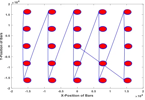
work, quality is defined using the results from an Ultimate Tensile Strength (UTS) test of each bar. Here, a UTS value of 1400 MPa represents an acceptable part while UTS values below 1400 MPa represent a faulty part (this definition is sufficient for demonstrating the feasibility of the proposed approach although it is noted that more complex criteria can be utilised in the future). Figure 2 shows the x-y coordinates of the laser during the build of 1 layer on the fusion bed.

Figure 2: x-y coordinates of the laser as a single layer of a build is being constructed. Red areas indicate the positions of the 25 tensile test bars while blue represents the laser path. Note that x-y coordinates are calculated from galvanometer measurements and that, for confidentiality reasons, units of position have been left as arbitrary.

Regarding the choice of sensing system, the general consensus amongst current literature is that data regarding melt pool characteristics will be closely related to build quality. Photodiode data is used to the current work as it is known to be closely correlated to properties of the melt pool (see [24], for example). While it has been hypothesised that, relative to thermal imaging systems, photodiodes may be able to capture data from a larger zone around the melt pool, the significance of this difference is currently unclear and could be investigated as future work.

4.1. Feature Extraction

bars per build). During each build, the x and y position of the laser was collected alongside time history measurements from 2 photodiodes sensors (sample frequency equal to 100kHz, resulting in approximately 400 GB of data per build). Here it is described how, from these large data, key features were extracted. This was based on the hypothesis that, from the photodiode measurements, it would be possible to extract relatively low dimensional fea-tures that give a statistically significant indication of build quality. It is also demonstrated how, because of the size of the data being utilised, feature ex-traction from SLM process measurements must be conducted using methods that are appropriate for large data sets.

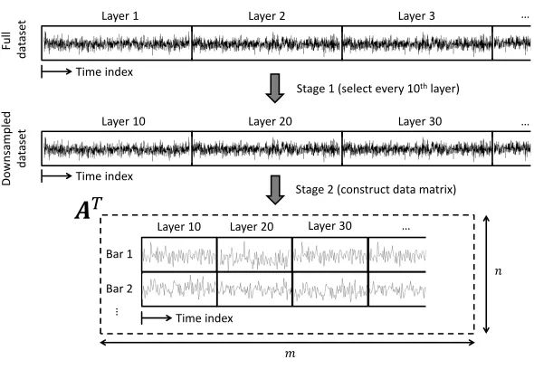
Initial data processing / reduction was conducted in two steps. Figure 3 graphically demonstrates this process for a single build (noting that the same procedure was applied to measurements from both photodiodes, Figure 3 illustrates the process for data from a single photodiode only). In Step 1, a downsampling procedure was used such that only the data from every 10th layer of the build was used in subsequent analyses2_{. Note that only} measure-ments taken when the laser was active were considered. In Step 2, for each layer that was analysed, the x-y position of the laser was used to identify which parts of each photodiode measurement time history corresponded to the building of a particular tensile test bar. This data was then collected together into an m×n data matrix, A, where the first column of A corre-sponded to measurements associated with bar one, the second column of A

corresponded to measurements associated with bar two etc. The transpose of A is illustrated graphically at the bottom of Figure 3.

2_{This step was taken simply to reduce the size of the data that needed to be}

Layer 1 Layer 2 Layer 3

Layer 10 Layer 20 Layer 30

…

…

Layer 10 Layer 20 Layer 30 …

Bar 1

Bar 2

…

Stage 1 (select every 10th_layer)

Stage 2 (construct data matrix)

࡭

Figure 3: Initial analysis of data from a single photodiode sensor, for a single build.

In the final step of the feature extraction procedure the intention was to apply a Singular Value Decomposition (SVD) to the data matrix, allowing

A to be written as the product of 3 matrices:

A=U DVT (22)

where U is an m×n orthogonal matrix, V is an n×n orthogonal matrix and

D= diag(σ1, ..., σm) (23)

where σ1, σ2, ... are constants (given by the eigenvalues of ATA) that, typ-ically, are ordered such that σ1 ≥ σ2 ≥ ... ≥ σm. The SVD allows each of the columns in A to be written as a linear combination of basis vectors. Specifically, writing B=DVT, it can be shown that

A=U B =⇒ aj =

n X

p=1

upBpj (24)

n constants (aj is associated with B1j, B2j, ..., Bnj etc.) It is these constants that can be used as features - inputs to the machine learning algorithm. In fact, by ordering the SVD results such that σ1 ≥ σ2 ≥ ... ≥ σm, close approximations ofAcan be realised without using the full set of basis vectors. Specifically, if a new matrix, A˜, is formed whose jth column is

˜

aj = ˜ n X

p=1

upBpj, n < n˜ (25)

then A˜ will form a low-rank approximation of A. Using A˜ instead of A

can therefore facilitate a reduction in the size of the feature space (in other words, the number of constants associated with each column of A˜ will be less than the number of constants associated with each column of A).

Unfortunately it was found that the matrixAwas prohibitively large for analysis via standard SVD. To circumvent this issue Awas, instead, decom-posed using a Randomised SVD. A brief outline of this procedure is given in the following text, however, for more information, readers may consult [47][48][49].

In the current work, for each tensile test bar, the time history of mea-surements from photodiodes 1 and 2 were each projected onto a single basis

vector only. As a consequence, each specimen becomes associated with a

2 2.5 3 3.5 4 4.5 5

Time index 104

2 3 4 5 6 7

Photodiode 1

Bar 1 (full data)

Bar 1 (projected onto 1 basis vector)

2 2.5 3 3.5 4 4.5 5

Time index 104

1.6 1.8 2 2.2 2.4 2.6 2.8 3 3.2 3.4

Photodiode 2

Bar 1 (full data)

Bar 1 (projected onto 1 basis vector)

Figure 5: Outputs for photodiode 2, for the first tensile test bar of build B4739. Black represents the uncompressed measurements, red represents measurements after they have been projected onto a single basis vector. Note that, for confidentiality reasons, unitless photodiode measurements are shown here.

4.2. Semi-Supervised Learning Application

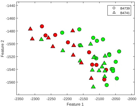
Tensile tests were performed on the builds using a standard Instron ten-sile machine at room temperature. As detailed in Section 4.1, the ultimate tensile strength (UTS) of the bars were used to define each bar as ‘acceptable’ or ‘faulty’. Semi-supervised learning was applied to the features extracted from each of the bars. However, bar 22 from build B4741 was not considered because its ultimate tensile strength could not be obtained. As a result, 49 specimens were considered in this analysis. Figure 6 shows the position of each specimen in the feature space and the associated labels. With the aim of distinguishing between ‘acceptable’ and ‘faulty’ cases, a GMM with two Gaussian distributions was employed.

proposed approach from the onset as, for approaches that are purely data based, knowing when a diagnosis is uncertain and where human intervention may be required will be crucial.

-2350 -2300 -2250 -2200 -2150 -2100 -2050 -2000

Feature 1

-1560 -1540 -1520 -1500 -1480 -1460 -1440

Feature 2

B4739 B4741

Figure 6: The position of each specimen in the feature space. The triangular points are for bars from build B4741 and the circular points are for bars from build B4739. The colour green represents acceptable specimens and red represents faulty specimens.

It is noted that, in the following, the algorithm is always initialised using the results of a purely supervised approach. Specifically, the first iteration ignores unlabelled samples and produces an initial estimate of the GMM parameters using the labelled samples only (employing equations (11), (12), (13) and (14)).

4.3. Results

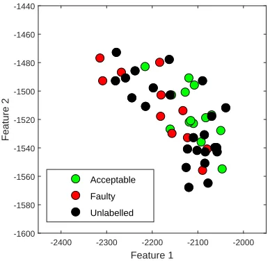
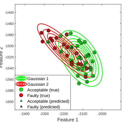
assigned to each specimen and triangles show the labels inferred by the al-gorithm. Note that the inferred labels are colour-coded depending on the probabilities that were assigned by the algorithm - purely green triangles correspond to the probability of a faulty specimen equal to zero while purely red triangles correspond to the probability of a faulty specimen equal to one.

-2400 -2300 -2200 -2100 -2000

Feature 1

-1600 -1580 -1560 -1540 -1520 -1500 -1480 -1460 -1440

Feature 2

Acceptable

Faulty

Unlabelled

-2400 -2300 -2200 -2100 -2000

Feature 1

-1600 -1580 -1560 -1540 -1520 -1500 -1480 -1460 -1440

Feature 2

Gaussian 1 Gaussian 2 Acceptable (true) Faulty (true) Acceptable (predicted) Faulty (predicted)

Figure 8: Example semi-supervised learning results. Red and green contours show the inferred geometry of the two Gaussian distributions in the mixture. Circles represent the true labels that were assigned to each specimen, while triangles show the inferred labels.

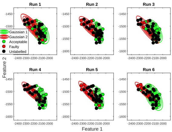
-2400-2300-2200-2100-2000 -1600 -1550 -1500 -1450 Feature 2 Run 1 Gaussian 1 Gaussian 2 Acceptable Faulty Unlabelled -2400-2300-2200-2100-2000 -1600 -1550 -1500 -1450 Run 2 -2400-2300-2200-2100-2000 -1600 -1550 -1500 -1450 Run 3 -2400-2300-2200-2100-2000 -1600 -1550 -1500 -1450 Run 4 -2400-2300-2200-2100-2000 Feature 1 -1600 -1550 -1500 -1450 Run 5 -2400-2300-2200-2100-2000 -1600 -1550 -1500 -1450 Run 6

Figure 9: Semi-supervised learning results obtained for 6 runs of a Monte Carlo simulation where, for each run, 24 unlabelled points are selected randomly.

55 60 65 70 75 80 85

% Success Rate

0 50 100 150 200 250 300 350 400 450 500

Frequency of Results

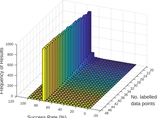
To analyse how the algorithms performance degrades as less labelled data is used, similar Monte Carlo simulations were conducted using different amounts of labelled and unlabelled data. Figure 11 shows results ranging from the case where there are 48 labelled points (and 1 unlabelled point) to the case where there are 20 label points (and 28 unlabelled points). While lower success rates are more frequently observed when the number of labelled data appoints is reduced (as one would expect), it is encouraging to note that algorithm performance does not drop off sharply. It can be seen, for example, that the number of labelled data points can be halved without significantly altering the resulting success rates. While, in the example, labels were rela-tively cheap to obtain (using tensile tests) the cost savings associated with the semi-supervised approach will clearly increase when more thorough and/or expensive certification methods are used. For example, in the author’s ex-perience, a CT scan of a typical component usually costs between £500 and

£1000.

20 22 24 26 28 30 32

No. labelled data points

34 36 38 0

200

40 120

400

100

Frequency of Results

42 600

80

Success Rate (%)

800

44 60

1000

40 ₂₀ 46

48 0

-20

5. Conclusion and Future Work

Additive Manufacturing (AM) is a digital approach for manufacturing highly customised components. However, uncertainties surrounding part quality hinders the adoption of AM technology in many risk-averse sectors. This paper is the outcome of a feasibility study wherein a semi-supervised machine learning algorithm was developed and applied to a large amount of AM process data (photodiode measurements, generated during SLM builds of tensile test bars). Key features were extracted from these large datasets us-ing a Randomised Sus-ingular Value Decomposition, before a Gaussian Mixture Model was trained to recognise builds that had been identified as ‘faulty’. The semi-supervised approach allowed this to be conducted using a reduced number of certification experiments and, even when the number of labelled data points was halved, could consistently identify faulty builds with a suc-cess rate close to 77%. Key contributions are summarised as follows:

1. In this work it was demonstrated how, when using machine learning to infer part quality from SLM process measurements, the large quantity of available data can prevent the application of ‘conventional’ feature extraction methods. It was illustrated how this challenge can be over-come using methods that are suitable for large datasets (a Randomised Singular Value Decomposition in this case).

2. By successfully classifying ‘successful’ builds with a 77% success rate, the feasibility of identifying faulty SLM builds using a purely data-based approach analysis of photodiode measurement time histories has been demonstrated.

3. It has been demonstrated that, through a semi-supervised approach, the number of costly certification experiments required in the imple-mentation of machine-learnt build classification can be significantly re-duced.

The paper has led to several avenues of future work.

feature extraction but will also increase the dimensionality of the feature space within which machine learning must be performed. Secondly, with regard to sensing systems, the current paper utilised data from photodi-odes sensors (which has been shown to be closely related properties of the melt pool [24]). Future work aims to investigate whether classification can be improved through the use of additional, complimentary sensing systems (acoustic sensors and thermal imaging cameras, for example). Finally, the authors are currently developing a version of the semi-supervised algorithm described in the current paper that is suitable for layer-by-layer defect de-tection, using data provided from CT scans. Ultimately, the aim of this work is to establish machine-learnt control strategies that can de-risk AM Tech-nology, facilitate its wider adoption and reduce the time associated with new materials innovation.

Acknowledgement

This work was conducted in the feasibility study ‘Towards Additive Man-ufacturing Process Control using Semi-Supervised Machine Learning’ that was funded through the EPSRC Network Plus Grant: Industrial Systems in the Digital Age EP/P001246/1, https://connectedeverything.ac.uk/.

References

[1] E. Uhlmann, R. Pontes, A. Laghmouchi, A. Bergmann, Intelligent pat-tern recognition of a SLM machine process and sensor data, Procedia CIRP 62 (2017) 464–469.

[2] P. O’Regan, P. Prickett, R. Setchi, G. Hankins, N. Jones, Metal based additive layer manufacturing: variations, correlations and process con-trol, Procedia Computer Science 96 (2016) 216–224.

[4] V. Renken, S. Albinger, G. Goch, A. Neef, C. Emmelmann, Development of an adaptive, self-learning control concept for an additive manufactur-ing process, CIRP Journal of Manufacturmanufactur-ing Science and Technology 19 (2017) 57–61.

[5] D. Lieber, M. Stolpe, B. Konrad, J. Deuse, K. Morik, Quality prediction in interlinked manufacturing processes based on supervised & unsuper-vised machine learning, Procedia Cirp 7 (2013) 193–198.

[6] N. Sadati, R. Chinnam, M. Nezhad, Observational data-driven model-ing and optimization of manufacturmodel-ing processes, Expert Systems with Applications 93 (2018) 456–464.

[7] J. Pang, Y. Gu, J. Xu, G. Yu, Semi-supervised multi-graph classification using optimal feature selection and extreme learning machine, Neuro-computing 277 (2018) 89–100.

[8] Y. Chen, B. Zhao, J. Zhang, Y. Zheng, Automatic segmentation for brain mr images via a convex optimized segmentation and bias field correction coupled model, Magnetic resonance imaging 32 (7) (2014) 941–955.

[9] Z. Ji, Y. Huang, Y. Xia, Y. Zheng, A robust modified gaussian mix-ture model with rough set for image segmentation, Neurocomputing 266 (2017) 550–565.

[10] B. Ribeiro, Support vector machines for quality monitoring in a plastic injection molding process, IEEE Transactions on Systems, Man, and Cybernetics, Part C (Applications and Reviews) 35 (3) (2005) 401–410.

[11] X. Liu, Q. Xu, J. Ma, H. Jin, Y. Zhang, Mslrr: a unified multiscale low-rank representation for image segmentation, IEEE Transactions on Image Processing 23 (5) (2014) 2159–2167.

[12] D. Montgomery, Statistical quality control, Vol. 7, Wiley New York, 2009.

[14] T. Spears, S. Gold, In-process sensing in selective laser melting (SLM) additive manufacturing, Integrating Materials and Manufacturing Inno-vation 5 (1) (2016) 2.

[15] T. DebRoy, H. Wei, J. Zuback, T. Mukherjee, J. Elmer, J. Milewski, A. Beese, A. Wilson-Heid, A. De, W. Zhang, Additive manufacturing of metallic components–process, structure and properties, Progress in Materials Science.

[16] G. Casalino, Computational intelligence for smart laser materials pro-cessing, Optics & Laser Technology 100 (2018) 165–175.

[17] S. Negi, S. Dhiman, R. Sharma, Determining the effect of sintering con-ditions on mechanical properties of laser sintered glass filled polyamide parts using rsm, Measurement 68 (2015) 205–218.

[18] R. Enneti, R. Morgan, S. Atre, Effect of process parameters on the selec-tive laser melting (SLM) of tungsten, International Journal of Refractory Metals and Hard Materials 71 (2018) 315–319.

[19] Y. Tian, D. Tomus, P. Rometsch, X. Wu, Influences of processing pa-rameters on surface roughness of hastelloy x produced by selective laser melting, Additive Manufacturing 13 (2017) 103–112.

[20] J. Tan, W. Wong, K. Dalgarno, An overview of powder granulometry on feedstock and part performance in the selective laser melting process, Additive Manufacturing.

[21] E. Olakanmi, R. Cochrane, K. Dalgarno, A review on selective laser sintering/melting (SLS / SLM) of aluminium alloy powders: Processing, microstructure, and properties, Progress in Materials Science 74 (2015) 401–477.

[22] X. Liu, M. Zeng, Y. Ma, M. Zhu, Wear behavior of al–sn alloys with dif-ferent distribution of sn dispersoids manipulated by mechanical alloying and sintering, wear 265 (11-12) (2008) 1857–1863.

[24] J. Kruth, P. Mercelis, J. Van Vaerenbergh, T. Craeghs, Feedback con-trol of selective laser melting, in: Proceedings of the 3rd international conference on advanced research in virtual and rapid prototyping, 2007, pp. 521–527.

[25] M. Mahesh, Y. Wong, J. Fuh, H. Loh, A six-sigma approach for bench-marking of rp&m processes, The International Journal of Advanced Manufacturing Technology 31 (3-4) (2006) 374–387.

[26] Y. Ning, Y. Wong, J. Fuh, H. Loh, An approach to minimize build errors in direct metal laser sintering, IEEE Transactions on automation science and engineering 3 (1) (2006) 73–80.

[27] C. Zhang, L. Li, A coupled thermal-mechanical analysis of ultrasonic bonding mechanism, Metallurgical and Materials Transactions B 40 (2) (2009) 196–207.

[28] C. Ning, F. You, Data-driven decision making under uncertainty in-tegrating robust optimization with principal component analysis and kernel smoothing methods, Computers & Chemical Engineering.

[29] A. Karimi, C. Kammer, A data-driven approach to robust control of multivariable systems by convex optimization, Automatica 85 (2017) 227–233.

[30] F. Tao, J. Cheng, Q. Qi, M. Zhang, H. Zhang, F. Sui, Digital twin-driven product design, manufacturing and service with big data, The International Journal of Advanced Manufacturing Technology (2017) 1– 14.

[31] Z. Ge, Review on data-driven modeling and monitoring for plant-wide industrial processes, Chemometrics and Intelligent Laboratory Systems.

[32] J. Wang, Y. Ma, L. Zhang, R. Gao, D. Wu, Deep learning for smart manufacturing: Methods and applications, Journal of Manufacturing Systems.

[34] M. Grasso, V. Laguzza, Q. Semeraro, B. Colosimo, In-process moni-toring of selective laser melting: spatial detection of defects via image data analysis, Journal of Manufacturing Science and Engineering 139 (5) (2017) 051001.

[35] M. Khanzadeh, S. Chowdhury, M. Tschopp, H. Doude, M. Marufuz-zaman, L. Bian, In-situ monitoring of melt pool images for porosity prediction in directed energy deposition processes, IISE Transactions (2018) 1–19.

[36] L. Scime, J. Beuth, Anomaly detection and classification in a laser pow-der bed additive manufacturing process using a trained computer vision algorithm, Additive Manufacturing 19 (2018) 114–126.

[37] M. Khanzadeh, S. Chowdhury, M. Marufuzzaman, M. Tschopp, L. Bian, Porosity prediction: Supervised-learning of thermal history for direct laser deposition, Journal of manufacturing systems 47 (2018) 69–82.

[38] G. Tapia, A. Elwany, H. Sang, Prediction of porosity in metal-based additive manufacturing using spatial gaussian process models, Additive Manufacturing 12 (2016) 282–290.

[39] C. Gobert, E. Reutzel, J. Petrich, A. Nassar, S. Phoha, Application of supervised machine learning for defect detection during metallic pow-der bed fusion additive manufacturing using high resolution imaging., Additive Manufacturing 21 (2018) 517–528.

[40] S. Shevchik, C. Kenel, C. Leinenbach, K. Wasmer, Acoustic emission for in situ quality monitoring in additive manufacturing using spectral convolutional neural networks, Additive Manufacturing 21 (2018) 598– 604.

[41] D. Ye, G. S. Hong, Y. Zhang, K. Zhu, J. Y. H. Fuh, Defect detection in selective laser melting technology by acoustic signals with deep belief networks, The International Journal of Advanced Manufacturing Tech-nology (2018) 1–11.

[43] J. Yu, C. Chaomurilige, M. Yang, On convergence and parameter se-lection of the em and da-em algorithms for gaussian mixtures, Pattern Recognition 77 (2018) 188–203.

[44] C. Bishop, Pattern Recognition and Machine Learning., Springer-Verlag New York, 2016.

[45] X. Hong, B. Huang, Y. Ding, F. Guo, L. Chen, L. Ren, Multi-model multivariate gaussian process modelling with correlated noises, Journal of Process Control 58 (2017) 11–22.

[46] J. Ma, J. Chen, W. Xiong, F. Ding, Expectation maximization esti-mation algorithm for hammerstein models with non-gaussian noise and random time delay from dual-rate sampled-data, Digital Signal Process-ing 73 (2018) 135–144.

[47] D. Achlioptas, Database-friendly random projections: Johnson-lindenstrauss with binary coins, Journal of computer and System Sci-ences 66 (4) (2003) 671–687.

[48] N. Halko, P. Martinsson, Y. Shkolnisky, M. Tygert, An algorithm for the principal component analysis of large data sets, SIAM Journal on Scientific computing 33 (5) (2011) 2580–2594.