Performance Evaluation of a New Proposed Variant of Fittest Job First Dynamic Round Robin (VFJFDRR) Scheduling Algorithm with Intelligent Time Slice

(1)

Volume 3, No. 3, May-June 2012

International Journal of Advanced Research in Computer Science

RESEARCH PAPER

Available Online at www.ijarcs.info

ISSN No. 0976-5697

Performance Evaluation of a New Proposed Variant of Fittest Job First Dynamic

Round Robin (VFJFDRR) Scheduling Algorithm with Intelligent Time Slice

Rakesh Mohanty*, Suchitra Panigrahi Department of Computer Science and Engineering

Veer Surendra Sai University of Technology Burla, Odisha, India

[email protected], [email protected]

Abstract—Round Robin (RR) is one of the most suitable and efficient scheduling algorithms for time-sharing systems. Recently many variants of RR scheduling algorithm have been developed and studied in the literature with the use of dynamic time quantum. In this paper, a new variant of Fittest Job First Dynamic Round Robin (FJFDRR) algorithm is proposed which we call as VFJFDRR in short. In this algorithm, the processes are arranged in the ready queue according to our calculated fit factor and are assigned dynamic time quantum using the intelligent time slice method. We have evaluated the performance and compared the results of our proposed VFJFDRR algorithm with the FJFDRR algorithm using three different cases of the input data set. Experimental results show that VFJFDRR performs better than FJFDRR in terms of average waiting time and average turnaround time when the processes are arranged in decreasing and random order of burst time. However VFJFDRR provides greater average waiting time and average turnaround time than FJFDRR when the processes are arranged in increasing order of burst time. In all the three cases, the number of context switches is increased for VFJFDRR making the algorithm more suitable for fair sharing.

Keywords: Operating System, Scheduling, Round Robin, Dynamic Time Quantum, Intelligent Time Slice.

I. INTRODUCTION

Operating system (OS) is an interface between an end user and system software. Recently emerging OS use the concepts of tasking, processing and multi-programming in order to achieve efficiency and improved system performance. Multi-tasking allows a user to perform more than one task at a time. Multiprocessing is the coordinated execution of programs by more than one processor. Multi-programming is the technique of executing several programs simultaneously in a single processor system. Scheduling refers to the way the processes are assigned to the processor. A scheduling algorithm is used for determining the sequence in which the processes will be dispatched to the processor so as to keep it busy. Design of efficient scheduling algorithms for OS with multi-tasking, multi-programming and multiprocessing environments is a major challenging research issue. Though many sophisticated scheduling algorithms have been designed, there is a scope for improvement for existing algorithms in the literature with a new strategy. In this paper our objective is to develop a new improved variant of a recently developed scheduling algorithm. In the next section we introduce some basic terminologies related to scheduling and operating system.

A. Basic Terminologies:

Prior to allocation to a processor the processes are put in a queue called ready queue. The time at which a process enters the ready queue is its arrival time. The amount of time a process spends waiting in the ready queue is called the waiting time. The time interval between the submission of a request by a process and the first response received is the response time. The processor time required to complete execution of a process is known as burst time. Turnaround time is the time duration from submission the submission of a process to its completion. Throughput is the number of processes that are completed per unit time. Processor

Utilization is a term used to describe how much the processor is busy or utilised. The number of times the processor switches from one process to another is called as the number of context switches.

The main goal of scheduling is to maximize processor utilization, throughput and minimization of response time, waiting time and turnaround time.

B. Well-Known Scheduling Algorithms:

The scheduling algorithms can be classified into two types such as non-preemptive and pre-emptive. A scheduling algorithm is non-preemptive, if once a process has been given the processor; the processor can not be taken away from that process. In case of pre-emptive algorithms, the processor can be taken away from the currently running process on the arrival of a higher priority process in the ready queue. First Come First Serve (FCFS), Shortest Job First (SJF) and Priority Scheduling algorithms are non-pre-emptive, where as Round Robin (RR) and Shortest Remaining Time Next (SRTN) are few widely used pre-emptive algorithms. We present below these algorithms.

(2)

Existing non-preemptive algorithms use only one of the basic parameters such as arrival time or user priority or burst time. Preemptive RR algorithm uses static time slice. These limitations of existing RR algorithm motivate us to design a new algorithm which uses more than one basic parameters and dynamic time quantum concept to improve the performance metrics of scheduling algorithms.

C. Related Work:

Various scheduling algorithms have been proposed in the literature along with comprehensive studies in [1] and [2]. Recently, many real time scheduling algorithms have been developed with dynamic time quantum. Best Job First (BJF) proposed in [3] combined the basic parameters of scheduling algorithms which includes burst time, user priority and arrival time of processes. Yaashuwanth. and et al.[4] have proposed an algorithm for real time systems to overcome the limitations of both Rate monotonic and Deadline monotonic algorithm by adding a Priority component. The static time quantum which is a limitation of RR was replaced with dynamic time quantum by Matarneh [5]. In FJFDRR [6] algorithm, dynamic time quantum has been calculated taking the median of the remaining burst time. The processes are scheduled giving importance to user priority and shortest burst time priority rather than using single parameter. Work done in paper [7], [8] and [9] have contributed a great deal towards soft real time systems. Dynamic time quantum is computed in the similar manner in [10] as in [6] but the processes are scheduled according to increasing order of shortest burst time only.

D. Our Contribution:

In this paper, the processes are arranged in the ready queue in a similar manner as in [6], but we are calculating dynamic time quantum using intelligent time slice to develop a variant of the FJFDRR algorithm. Intelligent time slice is calculated in the similar manner as in [7]. In our work, we have made a study of scheduling algorithms with a special focus on RR algorithm with dynamic time slice. We have proposed a new variant of FJFDRR algorithm, which we call as VFJFDRR. The pseudo code, flowchart and illustration of VFJFDRR have been presented. Using the performance metrics such as average turnaround time, average waiting time and number of context switches, we have evaluated the performance of FJFDRR and VFJFDRR. Our experiments involve three cases of data sets and computation of waiting time, turnaround time and number of context switches using Gantt chart.

E. Organization of the Paper:

In section II, the pseudo code, flowchart and illustration of our proposed algorithm is presented. Section III shows the results of experimental analysis of our algorithm and its comparison with FJFDRR. Conclusions and directions for future work are given in section IV.

II. OURPROPOSEDVFJFDRRALORITHM

In our proposed algorithm the processes are arranged in the ready queue according to the newly calculated Fit factor f and dynamic time slice is assigned to processes using intelligent time slice method.

A. Uniqueness of our Approach:

Generally with every process three factors are associated which are user priority, burst time and arrival time. Above factors play an important role in deciding the sequence in which the processes will be executed. Out of all these factors user priority plays the most significant role than burst time. Assigning different weights to these factors according to their importance we calculate the Fit factor f. Generally in RR algorithm, processes are taken from the ready queue in FCFS manner for execution. But in our algorithm, f is calculated for each process. The process having the lowest f value will be scheduled first. The criteria which will decide the early execution of the processes are higher user priority and shorter burst time.

As user priority has higher importance than burst time, so it is given a weight age of 60% and burst time is given 40%, weight age. We assume all the processes have same arrival time i.e. arrival time=0. Let User Priority, User Priority Weight, Shorter Burst time Priority, Burst time Priority Weight of the processes be denoted as PU, WUP , PSBT and WBTP respectively. Then Fit Factor f can be

calculated as

The performance of RR solely depends on the choice of time quantum. Our proposed algorithm makes use of dynamic intelligent time slice which allocates time quantum to each process independently based on the shortness component (SC), priority component (PC) and the context switch avoidance component (CSC). We formulate some relationships among the above parameters, which are being used in our proposed algorithm. PC for a process is given as 1 whose priority number is 1 and for the rest of the processes it is given as 0. Let Pi be the process id of ith

Context Switch Avoidance Component for process Pi

In the first round processes having SC value 1 are assigned full ITS as the time slice and for others, half the value of ITS is assigned. For successive rounds, the processes having SC value 1 are assigned a time quantum equal to double the value of time quantum in the previous round. For other processes, time slice is computed as the sum of time quantum and half the time quantum of previous round which can be used for current cycle.

.

B. Our Proposed Algorithm:

In our algorithm, all the processes are scheduled using the newly calculated Fit factor f. The process having the least f value will be scheduled first. Here intelligent time Slice method for dynamically assigning time slices to processes is used. We have used the following notations in our pseudo code for the VFJFDRR algorithm.

(3)

Let n  number of processes in the ready queue. f ( Pi ) fit factor for Pi

TBi  burst time of Pi Tq (Pi)  time quantum of Pi

TRB(Pi) remaining burst time of Pi

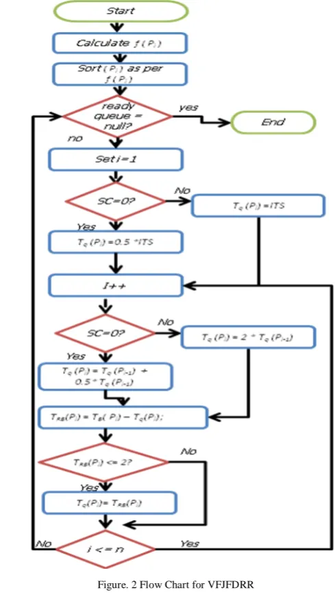
The pseudo code and flow chart of our proposed VFJFDRR algorithm are presented in Fig. 1 and Fig. 2 respectively.

Figure. 1 Pseudo code for VFJFDRR

Figure. 2 Flow Chart for VFJFDRR

C. Illustration:

Given the burst time of five processes as 1, 35, 12, 9 and 98 with user priority 5, 2, 4, 3 and 1 respectively. Then the fit factor f for each process is calculated as 3.4, 2.8, 3.6, 2.6 and 2.6 for P1 through P5 respectively using equation 1. After computing f, we arrange the processes in the ready queue according to increasing order of fit factor. Next, Intelligent time slice (ITS) component is calculated for each individual process depending on the shortness component (SC), priority component (PC) and context switch avoidance component (CSC). SC was calculated to be 0, 0, 1, 1, and 0. The PC was calculated to be 0, 0, 0, 0, and 1. Original time slice (OTS) was arbitrarily chosen as 12. Next OTS, PC and SC were added and their result subtracted from burst time. If the value comes to be less than OTS then it is assigned as the CSC component. Here the values are -11, 0, -1, -4, and 0. To calculate the ITS, all OTS, PC, SC and CSC are added together. In the First round, processes whose SC value is 1, i.e., for P3 and P4, are given the ITS value as their time quantum and for processes with SC value as zero, i.e., P1, P2, P5 are given half the value of ITS as their time quantum. In successive rounds processes P3 and P4 are given double their time quantum in the previous cycle and processes P1, P2 and P5 are assigned time 1. For i= 1, 2, 3 ….n, Calculate f ( Pi ).

2. Sort Pi for i=1,2,3, …n in ascending order

such that Pi < P j iff f ( Pi )< f ( Pj ) for i != j

3. while(ready queue != null)

for i=1 to n do

if ( i ==1) then

if(SCPi==0)then

Tq (Pi) =0.5 *TIS(Pi);

Else

Tq (Pi) = TIS(Pi);

End if

Else

If(SCPi==0)then

Tq (Pi) = Tq (Pi-1) + 0.5* Tq (Pi-1) ;

else

Tq (Pi) = 2 * Tq (Pi-1) ;

End if

TRB(Pi) = TB( Pi) – Tq(Pi);

If (TRB(Pi) <= 2 ) then

Tq(Pi)= TRB(Pi);

End if

End of for

End of while

4. Average waiting time, average turnaround time and number of

(4)

quantum equal to the sum of their previous time quantum and half the value of the previous time quantum. Remaining burst time for each processes is calculated and the time quantum is dynamically assigned to the remaining burst time based on some condition. Gantt Chart is prepared to determine the waiting time, turn around time and number of context switching for each process. Average waiting time, average turn around time is computed from the Gantt Chart.

III. PERFORMANCEEVALUATION&RESULTS

A. Assumptions:

In a uni-processor environment, all the experiments are performed and all the processes are independent. Time slice is assumed to be not more than the maximum burst time. The attributes like burst time, number of processes and the user-priorities of all the processes are known before submitting the processes to the processor. All processes are processor bound. No processes are I/O bound.

B. Experimental Frame work:

Our experiment consists of several input and output parameters. The input parameters consists of the number of processes, burst time, Original time slice (OTS), and user-priority. The output parameters consist of average waiting time, average turnaround time and number of context switches.

C. Data Set:

We have performed three experiments for evaluating performance of VFJFDRR and FJFDRR. For the experiments, we have considered three cases of data set. They are processes with burst time in decreasing, random order and increasing order respectively.

D. Performance Metrics:

The significance of our performance metrics are as follows:

a. Turnaround time (TAT): For the better performance of the algorithm, average turn-around time should be less. b. Waiting time (WT): For the better performance of the

algorithm, average waiting time should be less.

c. Number of Context switches (CS): For reducing the overheads of the operating system CS should be less while to attain fair sharing among the processes, CS should be high.

E. Experiments Performed:

In order to evaluate the performance of our proposed VFJFDRR algorithm and FJFDRR algorithm, we have taken a set of five processes in three different cases. Although for simplicity we have taken five processes, the algorithm works effectively for large number of processes. In each case, we have compared the experimental results of VFJFDRR algorithm with the FJFDRR algorithm presented in [3].

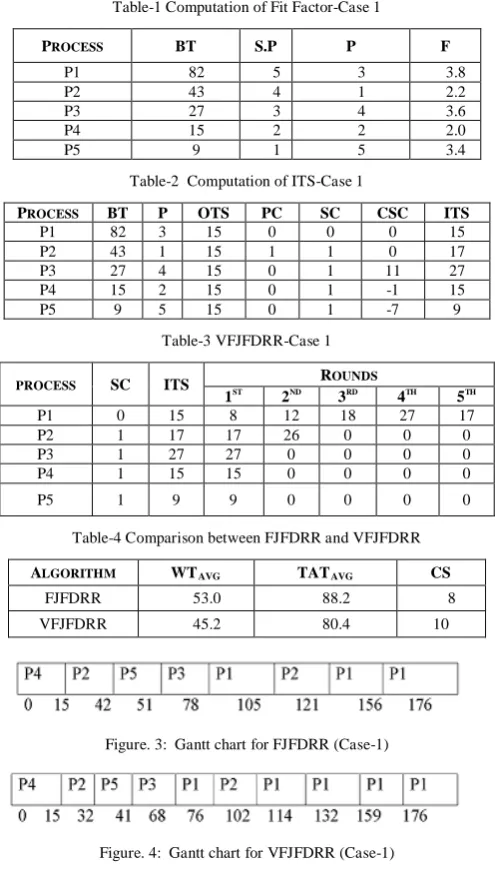
Case 1: We assume five processes P1, P2, P3, P4 and P5 are arriving at same with decreasing burst time 82, 43, 27, 15 and 9 respectively. The priorities assigned are 3, 1, 4, 2 and 5. The table-I, table-II and table-III show the output using algorithm FJFDRR and VFJFDRR. Table-IV shows the comparison between the two algorithms. Figure-3 and

Figure-4 shows Gantt chart for algorithms FJFDRR and VFJFDRR respectively.

PROCESS

Table-1 Computation of Fit Factor-Case 1

BT S.P P F

Table-2 Computation of ITS-Case 1

BT P OTS PC SC CSC ITS

Table-4 Comparison between FJFDRR and VFJFDRR

WTAVG TATAVG CS

FJFDRR 53.0 88.2 8

VFJFDRR 45.2 80.4 10

Figure. 3: Gantt chart for FJFDRR (Case-1)

Figure. 4: Gantt chart for VFJFDRR (Case-1)

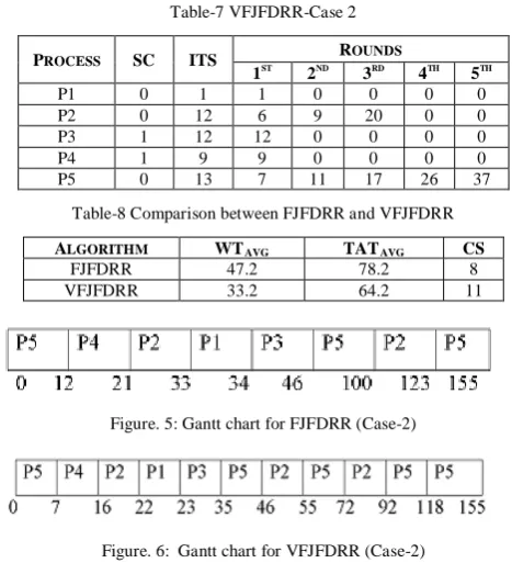
Case 2: We assume five processes P1, P2, P3, P4 and P5 are arriving at same with random burst time 1, 35, 12, 9 and 8 respectively. The priorities assigned are 5, 2, 4, 3 and 1. The table-V, table-VI and table-VII show the output using algorithm FJFDRR and VFJFDRR. Table-VIII shows the comparison between the two algorithms. Figure-5 and Figure-6 shows Gantt chart for algorithms FJFDRR and VFJFDRR respectively.

PROCESS

Table-5 Computation of Fit Factor -Case 2

BT S.P P f

(5)

PROCESS

FJFDRR 47.2 78.2 8

VFJFDRR 33.2 64.2 11

Case 3: We assume five processes P1, P2, P3, P4 and P5 are arriving at same with increasing burst time 9, 15, 27, 43 and 82 respectively. The priorities assigned are 5, 2, 4, 3 and 1. The table-IX, table-X and table-XI show the output using algorithm FJFDRR and VFJFDRR. Table-XII shows the comparison between the two algorithms. Figure-7 and Figure-8 shows Gantt chart for algorithms FJFDRR and VFJFDRR respectively.

Figure-9, figure-10 and figure-11 show the graph of average waiting time, average turnaround time and context switch respectively for FJFDRR and VFJFDRR.

PROCESS

BT P OTS PC SC CSC ITS

FJFDRR 53.0 88.2 8

VFJFDRR 65.4 100.6 15

0

Figure. 10: Graph for Avg. TAT

0

(6)

IV. CONCLUSIONS

From our experimental tabular and graphical results, we have observed that VFJFDRR algorithm is performing better than FJFDRR proposed in paper [6] in terms of average waiting time and average turnaround time when the processes are arranged in decreasing and random order of their burst time. However, when the processes are arranged according to increasing order of burst time FJFDRR gives better results as compared to VFJFDRR algorithm. We also observe that in VFJFDRR, the number of context switches increases thereby increasing the fair sharing among the processes. Developing a new and realistic variant of FJFDRR algorithm using arrival time and deadline can be a challenging work for future.

REFERENCES

[1] E.O. Oyetunji and et al. “Performance Assessment of some

Processor Scheduling Algorithms” Research Journal of Information and Technology, 1(1):22-26, 2009.

[2] A Pant “A Comparison between FCFS and Mixed

Scheduling” International Journal of Computer Science and Technology (IJCST), 2(2):076-079, 2011.

[3] Mohammed A. F. Al-Husain, “Best-Job-First Processor

Scheduling Algorithm”, Information Technology Journal 6 (2):288-293, 2007.

[4] Yaashuwanth and et al.”A New Scheduling Algorithm for

Real Time System”. International Journal of Computer Science and Information Security (IJCSIS), 6(2): 061-066, 2009.

[5] Rami J. Matarneh, “Self-Adjustment Time Quantum in

Round Robin Algorithm Depending on Burst Time of the Now Running Processes”, American Journal of Applied Sciences, 6 (10):1831-1837, 2009.

[6] Rakesh Mohanty and et al.”Design and Performance

Evaluation of a New Proposed Fittest Job First Dynamic Round Robin Scheduling Algorithm” International Journal of Computer Information Systems, 2(2): 054-060, 2011.

[7] Rakesh Mohanty and et al.”Priority Based Dynamic Round

Robin Algorithm with Intelligent Time Slice for Soft Real Time Systems”. International Journal of Advanced Computer Science and Applications (IJACSA), 2(2): 46-50, 2011.

[8] Yaashuwanth and et al.” Intelligent Time Slice for Round

Robin in Real Time Operating Systems” International Journal of Research and Reviews in Applied Sciences, 2(2): 126-131, 2010.

[9] H.S Behera and et al.” A New Dynamic Round Robin and

SRTN Algorithm with Variable Original Time Slice and Intelligent Time Slice for Soft Real Time Systems” International Journal of Computer Applications, 16(9), 2011.

[10] Rakesh Mohanty and et al.”Design and Performance