A New Boosting Multi class SVM Algorithm

Volume 4, No. 2, Jan-Feb 2013

International Journal of Advanced Research in Computer Science

RESEARCH PAPER

Available Online at www.ijarcs.info

A New Boosting Multi-class SVM Algorithm

Faculty of Computing and Informatics Multimedia University

Cyberjaya, Malaysia [email protected]

Yashwant Prasad Singh

Faculty of Computing and Informatics Multimedia University

Cyberjaya, Malaysia [email protected]

Abstract: Support Vector Machines (SVM) have originally designed for binary classification problems. However, Multi-class SVMs (MCSVM) are implemented by combining several binary SVMs. This paper presents a new boosting Multi-class SVMs (BmSVM) to overcome

computational complexity of existing construction MCSVM methods. The other two objectives of the paper are: first, to show therobustness of

BmSVM against different constructing Multi-class SVM methods such as One-Against-All, One-Against-One; Second, to compare the performance and complexity of BmSVM against SMO, AdaBoost, Decision Tree, and MCSVM. The simulation results demonstrate that the BmSVM on hypothyroid dataset with polynomial kernel is superior to the others.

Keywords: Boosting Multi-class SVM, Multi-class SVM , Boosting Algorithm, Boosting Multi-class SVM (BmSVM), SVM

I. INTRODUCTION

Support Vector Machines (SVMs) proposed by Vapnik [1] are a set of related supervised learning methods used for classification, regression and ranking. SVMs are classification prediction tools that use Machine Learning theory as a principled and very robust method to maximize predictive accuracy for detection and classification. SVMs can be considered as techniques which use hypothesis space of linear separators in a high dimensional feature space, trained with a learning algorithm from optimization theory that makes a learning bias derived from statistical learning theory [1, 2].

The SVM technique was developed to design separating hyperplanes for classification problems. In the 1990s SVM was generalized for constructing nonlinear separating functions and for real-valued functions approximation. Some applications of SVMs include text categorization, character recognition, bioinformatics, bankruptcy prediction, spam categorization and so forth [3].

The rest of the paper is organized as follows. In Section 2, SVMs classification is introduced and provides a formulation of linear and nonlinear SVM. Section 3 presents how Multi-class SVMs problem is solved through binary SVMs by deploying different methods. In Section 4 BmSVM is proposed and explained in detail and the experimental results are given in Section 5 to show the effectiveness of BmSVM over other classifiers which is followed by conclusion in Section 6.

II. SVMOVERVIEW

SVM classification is based on the idea of decision hyperplanes that determine decision boundaries in input space or high dimensional feature space. SVM constructs linear functions (hyperplanes either in input space or in feature space) from a set of labeled training dataset. This hyperplane will try to split the positive samples from the negative samples. The linear separator is commonly constructed with maximum distance from the hyperplane to the closest negative and positive samples. Intuitively, this causes correct classification for training data which is near, but not equal to the testing data.

Throughout training phase SVM takes a data matrix as input data and labels each one of samples as either belonging to a given class (positive) or not (negative). SVM treats each sample in the matrix as a row in an input space or high dimensional feature space, where the number of attributes identifies the dimensionality of the space. SVM learning algorithm determines the best hyperplane which separates each positive and negative training sample. The trained SVM can be deployed to perform predictions about a test samples (new) in the class.

Nonlinear problems in SVM are solved by mapping the

n- dimensional input space into a high dimensional feature space. Finally in this high dimensional feature space a linear classifier is constructed which acts as nonlinear classifier in input space. Most mathematical concepts as background materials for designing SVM and Multi-class SVM are introduced in the following [1, 4-11].

A. Linear Separable SVMs Classifier:

Consider a binary classification problem with N training samples (data). Each sample is indicated by a tuple (xi, yi)

and ( i = 1, 2, …, N), where xi=(xi1, xi2, …, xin) corresponds

to the attribute set for the ith sample. Conventionally let yi

∈{-1, 1} is considered as its class label. The decision boundary of a linear classifier (separator) can be written as follows:

wTx + b = 0, (1)

where w is weight vector and b is a bias term.

There are many linear separators, but the SVM design goal is to define a decision boundary that is maximally far away from any data point. This distance from the decision boundary to the closest data point determines the margin of the classifier. This technique of designing means that the decision boundary for an SVM is fully identified by a (generally small) portion of the data points which identify the position of the separator. These points are named support vectors. Fig. 1 shows the margin and support vectors for two classes problem.

If the training data are linearly separable then there exists a pair (w, b) such that:

wTxi+ b ≥ 1 if yi = 1, (2) wTxi+ b ≤ -1 if yi = -1, (3)

f(x) = sign(wTx + b). (4) For a given dataset and decision hyperplane, the functional margin of the ith sample xi with respect to a

hyperplane (w, b) is defined as in (5):

γi = yi(wTxi+ b) , (5)

The functional margin of a dataset of decision boundary is then twice the functional margin of any of the samples in the dataset with minimal functional margin (the factor of 2 comes from computing across the total width of the margin, as in Fig. 1). It is known that the shortest distance between a point and a hyperplane is perpendicular to the plane, and consequently, parallel to w. A unit vector in this direction is w/║w║. The maximum width of the band that can be designed for separating the support vectors of the two classes is known as geometric margin as shown in Fig. 1 by

ρ. Distance from any x_isample to the separator is equal to:

Designing linear separator is to maximize this geometric margin (6) in order to find the best w and b as formulated below:

ρ = 2 /║w║ is maximized,

For all (xi, yi), i =1, …, N ; s.t. yi (wTxi + b) ≥ 1. (7)

Figure 1. Decision boundary and margin of SVM.

Next step is optimizing quadratic function based on linear constraints. Quadratic optimization problems are a standard, popular class of mathematical optimization problems, and many algorithms is used for solving them. SVM classifiers construct using standard quadratic programming (QP) libraries. Therefore, the above problem is reformulated as minimization problem:

Φ(w) = ||w||= wTw is minimized,

for all (xi, yi), i =1,…,N : s.t. yi (wTxi+ b)≥ 1. (8)

The solution for the above problems includes constructing a dual problem where a Lagrange multiplier αi

is linked with every inequality constrains (yi (wTxi+ b)≥ 1)

in the primal problem: Find α1, …, αN such that

is maximized with respect to αi subject to the following constraints:

The solution of the dual problem αi must satisfy the condition αi{yi (wTxi- b) -1)} = 0 for i =1, 2, …, N.

Then solution to the primal is:

In the solution above, most of αi are zero for data

samples which are not support vectors. Each non-zero αi

specifies that the equivalent xi is a support vectors. So the

classification function is given as below:

We don’t need w explicitly in (11) since it relies on an inner product between the test point x and the support vectors xi. Finding class label for any data points xj involves

computing the inner products xiTxj .

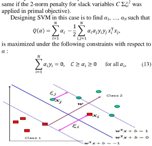
B. Linear Non-Separable SVMs Classifier:

We have presented above, where dataset are linearly separable, and what we present below is the data which is not linearly separable. The standard approach is to allow the fat decision boundary as shown in Fig. 2 to make a few mistakes (some points - outliers or noisy samples - are inside or on the wrong side of the margin). We then pay a cost for each misclassified sample, which depends on how far it is from meeting the margin requirement given in (8). To implement this, slack variables ξi are introduced below.

The formulation of the SVMs optimization problem with slack variables is given below:

Find w, b and ξi≥ 0 such that

For all (xi, yi), i =1, ..., N : s.t. yi (wTxi+ b)≥ 1 – ξi, , (12)

The parameter C is a regularization term, which can be viewed as a way to control overfitting, it is trade-off between the relative importance of maximizing the margin and fitting the training data.

Dual problem is same as separable case (would not be same if the 2-norm penalty for slack variables C Σξi2 was applied in primal objective).

Designing SVM in this case is to find α1, …, αN such that

is maximized under the following constraints with respect to

α :

Figure 2. Slack variables for linearly nonseparable data.

constant C which bound the possible size of the Lagrange multipliers for the support vector data points. Like before, the xi with non-zero αi is the support vectors. The solution of

the dual problem is of the form:

The solution of the dual problem αi must satisfy the condition αi{yi (wTxi - b) -1) + ξi } = 0 for i =1, 2, …, N.

Again, we don’t need to compute w explicitly for classification function as shown in (15):

C. Nonlinear SVMs Classifier:

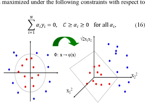
In SVMs the optimal hyperplane is defined to maximize the generalization. But if the training data are not linearly separable, the designed classifier may not have high generalization ability, even though the hyperplanes are determined optimally. So to improve linear separability, the original input space is mapped into a high dimensional space which is known as feature space [4].

SVMs present an easy and efficient way of performing this mapping to a higher dimensional space, which is called the kernel trick [2]. The SVMs linear classifier depends on a dot product between data point vectors. Assume we transform the data to some (possibly infinite dimensional) space H via a mapping function Φ such that the data appear in the form of Φ(xi)TΦ(xj). Linear operation in H is alike to non-linear operation in input space, while x = (x1, x2) and

Ф(x) =(x12, x22, √2x1x2) Fig. 3 illustrates this mapping. Let K(xi, xj)=Ф(xi)TФ(xj) as a kernel function, so we

change all inner products to kernel functions for training data.

Designing SVM is to find α1 ,…, αN such that

is maximized under the following constraints with respect to

α

Figure 3. Nonlinear SVMsdecision boundary.

Then the classifier is as below:

The four commonly used families of kernels are: a. Linear kernel

K(xi, xj) = xiTxj

b. Polynomial kernel with degree d K(xi, xj) = ( xiTxj + 1)d

c. Radial basis function (RBF) kernel (σ is a positive parameter for controlling the radius)

K(xi, xj) = exp (-|| xi- xj||2 / 2σ2)

d. Sigmoid kernel (δ is a positive parameter)

K (xi, xj) = tanh (δxiTxj + r)

III. MULTI-CLASSSVMS(MCSVM)

In case of Multi-class classification problems, the issue becomes more complex because the outputs could be more than one class and must be divided into M mutually exclusive classes. In fact, there are many ways to solve Multi-class classification problems for SVM such as Directed Acyclic Graph (DAG), Binary Tree (BT), One-Against-One (OAO) and One-Against-All (OAA) classifiers.

A. Directed Acyclic Grapph SVM (DAGSVM):

Directed acyclic graph SVM (DAGSVM) is introduced by Platt, Cristianini [12]. It works like OAO method in training stage by constructing M × (M-1)/2 binary classifiers. In recognition (testing) stage it uses a rooted binary directed acyclic graph which includes M leaves and

M × (M-1)/2 nodes (comprising of a binary SVM form ith

and jth class). For a test sample, evaluation of binary decision function starts at the root node; afterward its movement to either left or right side depends on the output value.

B. Binary Tree of SVM (BTSVM):

This technique deploys multiple SVMs arranged in a binary tree structure [13]. Every SVM in its related node of the tree is trained by using two of the classes. The measurement of similarity between the two classes and the remaining samples is made by deploying probabilistic outputs. All existing samples in the node are allocated to the two consequent subnodes of the previously chosen classes by similarity and this step iterates at every node until all sample of each node belong to one class. The drawbacks of this technique are high training time and low performance in huge training dataset; since all samples of every node should be tested to define their classes during constructing tree.

C. One-Against-One SVM (OAOSVM):

OAOSVM constructs M × (M -1)/2 binary classifiers, using all the binary pair-wise combinations of the M classes. Each classifier is qualified by using the examples of the first class as positive and the examples of the second class as negative examples. To combine these classifiers, the Max Wins algorithm is accepted. The subsequent class is determined by selecting the class voted by the majority of the classifiers. The number of examples used for training each one of the OAOSVM classifiers is smaller, since only examples from two of all M classes are considered. The smaller number of examples makes shorter training times [8, 14].

s.t.

.

After all M × (M -1)/2 classifiers are designed, the Max Wins strategy is deployed in this way: if the result of

assigns the ith class to x then the vote of the ith class is increased by one; otherwise, vote of the jth class is added by one. So, the class with the largest vote will be assigned to x.

D. One-Against-All SVM (OAASVM):

In case of M-class problems (M >2), M binary SVM classifiers are constructed [8, 15]. The ith SVM is trained such that the samples in the ith class are labeled as positive samples and all the rest as negative samples. In the recognition stage, a test sample is obtained from all M

SVMs and is labeled according to the maximum output among the M classifiers.

The Multi-class SVM (MCSVM) problem is solved by constructing a decision bounary by given N samples typically with noise: (x1, y1), …, (xN, yN ), where xi : i = 1,

…, N is a vector of length n and yi∈ {1, …, M} represents

the class of the sample. The classical approach to solve MCSVM classification problems is to consider the problem as a collection of binary classification problems. The OAA method constructs M classifiers, one for each class. The ith

classifier constructs a hyperplane between class i and the M

– 1 remaining classes. A new test sample is allocated to the class that the distance from the margin, in the positive direction, is maximal.

We can generalize optimization problem [1] to the following by minimizing:

s.t.

ξij≥ 0 , for i = 1, …, N . Here the training sample xi is mapped to feature space

(high dimensional space) using function Φ and C is defined as trade-off parameter.

Minimizing is equal to maximize

which means the margin between two classes. In case of non linear separable samples, presence of trade-off term

is necessary for reducing the training error rate. There is an essential need to balance the training errors and the regularization term .

The following M decision boundaries emerge as a result of solving equation (19),

, . . .

.

So, the sample xi is assign to the class with the largest

decision boundary’s value as follows

. (20)

Therefore, the dual problem with N-variable and M

quadratic optimization problems with N-variable should be solved correspondingly.

IV. BMSVMALGORITHM

The main goal of any boosting algorithms is to improve existing classification algorithm in order to enhance its accuracy. This section presents a new boosting technique for SVM classifiers by investigating two ways of boosting SVMs as well as their combinations:

a. Creating weak SVMs for different values of C on the same dataset and finding majority sign defines the class label for input data.

b. Integrating existing AdaBoost with SVM using weighted training dataset and weighted voting.

The critical problem that we face in these two methods is computational complexity in real world problem. The most possible solution is to reduce number of the samples used for designing the base classifiers. The proposed boosting SVM, BmSVM (Boosting Multi-class SVM), involves designing multiple binary SVM based on selection of disjoint subset of dataset from whole dataset (training set), and then combining them for calculating majority sign for classification.

Support Vectors (SV) are those important samples (due to its limited number in compared to number of training samples) which are used for constructing classifiers. Finding SVs among all training samples are other problems which is very complicated because we need to use all training samples to solve quadratic optimization problem. We can reduce computations by selecting important samples instead of original training set and finding the SVs among these selected training samples. The usefulness and importance of training sample is defined by the location of sample related to the separating hyperplane. In addition to SVs, the samples that are closest to separator, especially those samples that lie in classification margin would be important and should be included in selected training set to find SVs. In the case that there are no samples exist in the classification margin we can change weighted SVM dynamically by changing training set to get important sample in order to find different SVs. To improve accuracy of classification in this step we consider combination of boosting classifiers[16].

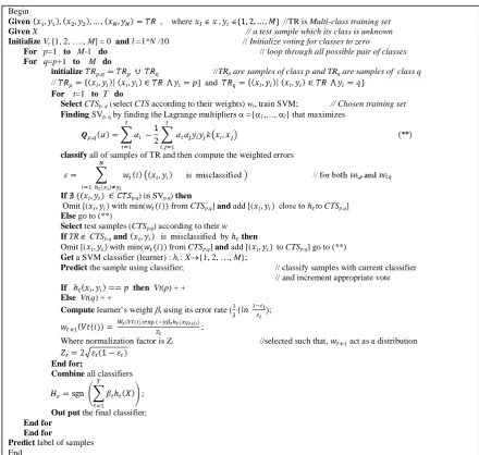
While, we convert Multi-class SVMs to binary SVMs by employing any available methods, as it described in Section 3, then, we can extend the aforementioned instruction to solve Multi-class SVMs classification problem. Fig. 4 shows detail of the proposed BmSVM algorithm and is summarized as below:

combine all the genrated classifiers of T rounds by considering majority voting sterategy.

Begin

Given , where //TR is Multi-class training set

Given X // a test sample which its class is unknown

Initialize Vt[1, 2, …., M] = 0 and l =1*N /10 // Initialize voting for classes to zero

For p=1 to M-1 do // loop through all possible pair of classes

For q=p+1 to M do

initialize //TRp are samples of class p and TRq are samples of class q

// and

For t=1 to T do

Select CTSp, q (select CTS according to their weights) wt, train SVM; // Chosen training set

Finding SVp, q by finding the Lagrange multipliers α ={α1,…, αl} that maximizes

classify all of samples of TR and then compute the weighted errors

If p,q) in SVp,q) then

Omit [( with min( from CTSp,q] and add [( to CTSp,q]

Else go to (**)

Select test samples (CTSp,q) according to their w

If TR∉ CTSp,q and by then

Omit [( with min( from CTSp,q] and add [( to CTSp,q] go to (**)

Get a SVM classifier (learner) : ht : X→{1, 2, …, M};

Predict the sample using classifier; // classify samples with current classifier // and increment appropriate vote If then Vt(p) + +

Else Vt(q) + +

Compute learner’s weight βt using its error rate ( ;

;

Where normalization factor is Zt //selected such that, act as a distribution

End for;

Combine all classifiers

Out put the final classifier; End for

End for

Predict label of samples End

Figure 4. Pseudo code for the proposed BmSVM algorithm.

V. EXPERIMENTALRESULTS

Thyroid gland sprinkles thyroid hormones to assist the regulation of the body's metabolism. The abnormalities of secretion thyroid hormones are divided into two groups of problem (hypothyroidism and hyperthyroidism) [17].

In this section, we provide experimental results on hypothyroid dataset from UCI repository [18] for the proposed BmSVM. Computational results for the CPU time and accuracy of BmSVM with other algorithms in Weka [19] are provided to evaluate the effectiveness of BmSVM.

Hypothyroid dataset had 4 classes with 30 attributes. The number of samples of given data was 3772 which is divided to 3167 samples as the training data and 605 as the test data. The robustness of BmSVM classifier in compare with other classifiers was done on this dataset by applying different kernels to determine its accuracy and complexity.

A. Effect of Kernel Functions:

The performance of BmSVM greatly depends on the choice of the kernel functions (to transform data from input space to a higher dimensional feature space). There are no

definite rules for this selection except satisfactory performance by simulation study.

Table 1: Comparison of three different kernels

Kernel C Accuracy Computation Time Training Test Training Test

Linear 10 93.8% 92.5% 58.8s 52.9s 40 94.1% 93.8% 92.2s 93.3s 60 97.2% 96.4% 40.74s 40.21s 80 93.4% 92.9% 123.9s 134.6s Polynomial 10 95.4% 94.2% 416.7s 413.6s 40 96.6% 95.1% 656.5s 620s 60 99.1% 96.9% 139.54s 134.5s 80 97.3% 95.2% 711.6s 783.7s RBF 10 92.4% 93.1% 152.9s 155.8s 40 93.1% 92.2% 135.3s 139.1s 60 95.5% 96.1% 50.48s 79.49s 80 92.3% 92% 186s 187.7s

kernel in our expriment is 3. In spite of better accuracy for polynominal kernel as in Table 1, the computation time for classifying the samples in RBF kernel is half of polynominal kernel.

B. Effect of Using Methods in MCSVM:

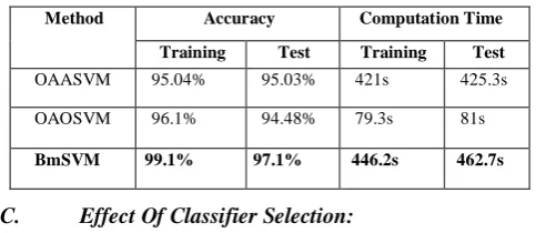
We examined the efficiency of different methods on MCSVMs using the OAOSVM, OAASVM and BmSVM methods with polynomial kernels by setting d=3 and trade-off (balance between slack variables and regularization parameter) as C = 60. This value (60) is determined by conducting many experiments for different values. The classification results are shown in Table 2. The result shows that the BmSVM has better performance than OAOSVM and OAASVM, but it takes long time to construct classifier and test sample.

Table 2: Robustness of BmSVM method

Method Accuracy Computation Time

Training Test Training Test OAASVM 95.04% 95.03% 421s 425.3s

OAOSVM 96.1% 94.48% 79.3s 81s

BmSVM 99.1% 97.1% 446.2s 462.7s

C. Effect Of Classifier Selection:

The robustness and efficiency of BmSVM classification is shown by comparing the experimental result of the BmSVM with MCSVM, Decision Tree and AdaBoost. The results are presented in Table 3 and it shows the BmSVM superiority over other classifiers.

Table 3: Average classification accuracy result of different algorithms Classifier Accuracy Computation Time

Training Test Training Test MCSVM 99.1% 96.9% 131.82s 141.6s

Decision Tree (J48) 95% 94.1% 0.11s 0.22s

AdaBoost 96.4% 95.5% 0.29s 0.39s

BmSVM 99.1% 97.1 565s 516.9s

VI. CONCLUSION

This paper presented the BmSVM as a new boosting algorithm for enhancing the accuracy and performance of common Multi-class SVM. The performance of BmSVM algorithm by selecting different kernels is examined on hypothyroid dataset. The experimental results demonstrated the superior performance and accuracy of BmSVM over MCSVM, Decision Tree, and AdaBoost.

VII. REFERENCES

[1]. Vapnik VN. The Nature of Statistical Learning Theory.

New York: Springer-Verlag 1995.

[2]. Scholkopf B, Smola AJ. Learning with Kernels: Support

Vector Machines, Regularization, Optimization, and Beyond: MIT Press; 2001.

[3]. Boser BE, Guyon IM, Vapnik VN. A Training Algorithm

for Optimal Margin Classifiers. Proceedings of the fifth annual workshop on Computational learning theory.

Pittsburgh, Pennsylvania, United States: ACM; 1992. p. 144-52.

[4]. Abe S. Support vector machines for pattern classification.

London -Verlag: Springer; 2006.

[5]. Burges CJC. A Tutorial on Support Vector Machines for

Pattern Recognition. Data Min Knowl Discov. 1998;2:121-67.

[6]. Hong J-H, Cho S-B. A Probabilistic Multi-Class Strategy

of One-vs.-Rest Support Vector Machines for Cancer Classification. Neurocomput. 2008;71:3275-81.

[7]. Hsu C-W, Chang C-C, Lin C-J. A Practical Guide to

Support Vector Classification. Department of Computer Science, National Taiwan University; 2003.

[8]. Hsu C-W, Lin C-J. A comparison of methods for multiclass

support vector machines. Neural Networks, IEEE Transactions on. 2002;13:415-25.

[9]. Tan P-N, Steinbach M, Kumar V. Introduction to Data

Mining, (First Edition): Addison-Wesley Longman Publishing Co.; 2005.

[10]. Weston J, Watkins C. Support Vector Machines for

Multi-class Pattern Recognition. the 7th European Symposium on Artificial Neural Networks. Bruges, Belgium1999. p. 219-24.

[11]. Muller KR, Mika S, Ratsch G, Tsuda K, Scholkopf B. An

introduction to kernel-based learning algorithms. Neural Networks, IEEE Transactions on. 2001;12:181-201.

[12]. Platt JC, Cristianini N, Shawe-Taylor J. Large Margin

DAGs for Multiclass Classification. Advances in Neural Information Processing Systems: MIT Press; 2000. p. 547-53.

[13]. Dietterich TG, Bakiri G. Solving Multiclass Learning

Problems Via Error-Correcting Output Codes. Journal of Artificial Intelligence Research. 1995;2:263-86.

[14]. Peng X, Chan AK. Support vector machines for multi-class

signal classification with unbalanced samples. International Joint Conference on Neural Networks2003. p. 1116-9.

[15]. Vapnik VN. Statistical learning theory. New York: Wiley;

1998.

[16]. Diao L, Hu K, Lu Y, Shi C. A Method to Boost Support

Vector Machines. Proceedings of the 6th Pacific-Asia Conference on Advances in Knowledge Discovery and Data Mining: Springer-Verlag; 2002. p. 463-8.

[17]. Saiti F, Naini AA, Shoorehdeli MA, Teshnehlab M.

Thyroid Disease Diagnosis Based on Genetic Algorithms Using PNN and SVM. 3rd International Conference on Bioinformatics and Biomedical Engineering (ICBBE 2009)2009. p. 1-4.

[18]. Frank A, Asuncion A. UCI Machine Learning Repository.

[http://archiveicsuciedu/ml]: Irvine, CA: University of California, School of Information and Computer Science 2010.

[19]. Hall M, Frank E, Holmes G, Pfahringer B, Reutemann P,