Surface Reconstruction from Noisy and Sparse Data

(1)

Scholarship@Western

Electronic Thesis and Dissertation Repository

12-7-2015 12:00 AM

Surface Reconstruction from Noisy and Sparse Data

Mark A. Brophy

The University of Western Ontario Supervisor

Dr. John Barron

The University of Western Ontario Joint Supervisor Dr. Steven Beauchemin

The University of Western Ontario Graduate Program in Computer Science

A thesis submitted in partial fulfillment of the requirements for the degree in Doctor of Philosophy

Follow this and additional works at: https://ir.lib.uwo.ca/etd

Part of the Other Computer Sciences Commons

Recommended Citation Recommended Citation

Brophy, Mark A., "Surface Reconstruction from Noisy and Sparse Data" (2015). Electronic Thesis and Dissertation Repository. 3375.

https://ir.lib.uwo.ca/etd/3375

This Dissertation/Thesis is brought to you for free and open access by Scholarship@Western. It has been accepted for inclusion in Electronic Thesis and Dissertation Repository by an authorized administrator of

(2)

from

Noisy and Sparse Data

by

Mark Brophy

Faculty of Science

Department of Computer Science

Submitted in partial fulfillment

of the requirements for the degree of

Doctor of Philosophy

School of Graduate and Postdoctoral Studies

The University of Western Ontario

London, Ontario, Canada

c

(3)

We introduce a set of algorithms for registering, filtering and measuring the similarity of unorganized 3D point clouds, usually obtained from multiple views.

We contribute a method for computing the similarity between point clouds that represent closed surfaces, specifically segmented tumours from CT scans. We obtain watertight surfaces and utilize volumetric overlap to determine similarity in a volumetric way. This similarity measure is used to quantify treatment variability based on target volume segmentation both prior to and following radiotherapy planning stages.

We also contribute an algorithm for the drift-free registration of thin, non-rigid scans, where drift is the build-up of error caused by sequential pairwise registration, which is the alignment of each scan to its neighbour. We construct an average scan using mutual nearest neighbours, each scan is registered to this average scan, after which we update the average scan and continue this process until convergence. The use case herein is for merging scans of plants from multiple views and registering vascular scans together.

Our final contribution is a method for filtering noisy point clouds, specif-ically those constructed from merged depth maps as obtained from a range scanner or multiple view stereo (MVS), applying techniques that have been utilized in finding outliers in clustered data, but not in MVS. We utilize ker-nel density estimation to obtain a probability density function over the space of observed points, utilizing variable bandwidths based on the nature of the neighbouring points, Mahalanobis and reachability distances that is more dis-criminative than a classical Mahalanobis distance-based metric.

(4)

A special thank you to my supervisor Dr. John Barron, you’ve been

in-finitely helpful, patient and caring. Having someone to learn from and bounce

ideas off has been invaluable. You are simultaneously pragmatic and creative

in your approach to problem solving. Likewise, thank you to my co-supervisor

Dr. Steven Beauchemin, you gave me guidance and room to experiment from

the very beginning, allowing me to explore and truly understand and own the

process of my postgraduate studies. Penning publications with both of you

has been an honour. Thank you to Spencer Martin and Ayan Chaudhury, you

both have been fantastic collaborators.

Thank you to my partner Erika, you have always been loving, supportive

and proud. Even at the lowest points of my research, you have never

enter-tained the idea of giving up. Similarly, thank you to my mother and father,

you have been incredible throughout this entire process. All three of you have

overlooked my glaring shortcomings and helped me move forward on more

occasions than I can count. Thank you to Dr. Paul Azzopardi, Sam Hinds,

Jonathan Hornell-Kennedy and everyone at the London Western Track and

Field Club for making London my home for many years.

Thank you to all of the great scientists at Western who have inspired me,

but especially those in my area: in addition to supervisors John and Steven,

thank you to Drs. Yuri Boykov, Olga Veksler and Mahmoud R. El-Sakka. You

all continue to show me what ambitious, top notch vision research looks like.

Thank you to the members of my committee, Drs. John Zelek, Ken A.

McIsaac, Mahmoud El-Sakka and Charles Ling: I know that your schedules

are absurdly busy at this time of year and I appreciate your commitment to

both my personal growth and academe at large.

(5)

ABSTRACT ii

ACKNOWLEDGEMENTS iii

CONTENTS iv

LIST OF TABLES vii

LIST OF FIGURES viii

1 Introduction 1

1.1 Contributions . . . 2

1.2 Publications . . . 3

1.3 Overview of Thesis . . . 4

2 Energy based surface reconstruction for point clouds 7 2.1 Preliminaries: Minimization, Smoothing and Segmentation . . 9

2.2 Level Sets and Snakes . . . 11

2.2.1 Geodesic Active Contours . . . 12

2.3 Graph Cuts . . . 13

2.3.1 Multiview Graph Cuts . . . 14

2.4 Total Variation . . . 16

2.4.1 Total Variation Surface Reconstruction . . . 17

2.5 Chan-Vese: Active Contours without Edges . . . 18

2.5.1 Shape Priors in Level Set Formulations . . . 19

2.6 Segmentation of Point Clouds with Level Sets . . . 21

2.7 Flux-based Functionals . . . 21

2.7.1 Continuous Global Optimization . . . 24

2.7.2 Global Minimization for Shape Fitting . . . 25

2.7.3 Power Watersheds . . . 25

2.8 Summary of Methods . . . 27

(6)

3.1 Introduction . . . 28

3.2 Background . . . 30

3.3 Problem . . . 31

3.4 Methodology . . . 32

3.5 Point Cloud Construction . . . 35

3.5.1 Surface Fitting . . . 36

3.5.2 Computing Normals . . . 38

3.5.3 Minimal Surface Fitting to Segmented Point Cloud . . 39

3.6 Similarity Quantification . . . 41

3.7 Results . . . 42

3.8 Conclusions and Future Work . . . 47

4 Global Registration of Multiple Thin Structures 50 4.1 Previous Work . . . 54

4.2 Proposed Method . . . 57

4.2.1 Approximate Alignment . . . 60

4.2.2 Global Non-Rigid Registration via MNN . . . 60

Global Registration . . . 60

4.3 Results . . . 61

4.3.1 Synthetic Vascular Data . . . 61

4.3.2 Plant Data . . . 62

5 Kernel Density Filtering for Noisy Point Clouds in One Step 70 5.1 Introduction . . . 71

5.2 Previous Work . . . 73

5.3 Obtaining a Probability Density Function from Measured Data 77 5.3.1 Kernel Density Functions . . . 78

5.3.2 Mahalanobis Distance . . . 78

5.3.3 Local Bandwidth Estimation . . . 80

5.4 Methodology . . . 80

5.4.1 Reachability Distance . . . 81

5.5 Kernel Density Filtering on Data with Additive Noise . . . 82

5.6 Results . . . 83

(7)

6.2 Future Work . . . 91

BIBLIOGRAPHY 92

VITA 100

(8)

3.1 Coefficient of Variation for VOE. . . 47

4.1 Quantitative results for different algorithms and data sets. . . 57

5.1 Confusion matrix describing the different classifications of in-liers and outin-liers. . . 83

(9)

2.1 Level set segmentation of a 2D point cloud. . . 22 2.2 Level set segmentation of a 3D point cloud of a cube. . . 23

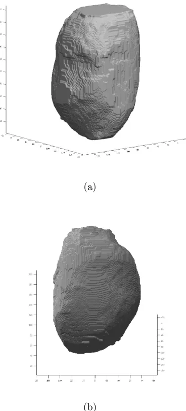
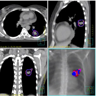
3.1 Two different views of the same segmented primary GTV. Note the top of the surface is flat and this made the volume fitting more challenging because the flux width has to be wider to ensure that the entire surface is contained. The flat top is visible in (a). . . 33 3.2 Slices of physician provided segmentations for patient E. The

GTVs on different axes are shown at top left, top right and bottom left, while the bottom right image shows the superim-posed 3D meshes for all segmentations. Top left shows a slice at

z = 52.7, top right shows slicex = 5.62 and bottom left shows slice y=−18.485. . . 34 3.3 Point cloud extracted from physician segmentations. . . 35 3.4 Approximate meshed surface for point cloud seen in Figure 3.3,

as fitted using the ball pivoting algorithm. . . 37 3.5 Normals calculated for an approximate surface. . . 38 3.6 Three different segmentations of patient 3’s nodal tumour by

different physicians. . . 43 3.7 Six segmentations of patient 3’s primary tumour by different

physicians. . . 44 3.8 Graph of volumetric overlap for gated tumours for each patient. 45 3.9 Graph of RMS distance for gated tumours for each patient. . . 45 3.10 Slices of physician provided segmentations for patient B GTV

on different axes are shown at top left, top right and bottom left, while bottom right shows the superimposed 3D meshes for all segmentations. Top left shows a slice at z = 53.400, top right shows slice x = −5.313 and bottom bottom left shows a slice aty =−17.808. . . 49

(10)

to obtain our data set. . . 52 4.2 Pairwise registration results for two scans of the Stanford Bunny.

Top row: original two views, Bottom row: results obtained us-ing Rusu et al. (FPFH) [61], Fitzgibbon (LMICP) [23], Jian and Vemuri (GMMReg) [33] and Myronenko and Song (CPD)

[49]. . . 57 4.3 Pairwise registration results two scans of the real Arabidopsis

plant data. Top row: the original two views. Bottom row: results obtained using Rusu et al. [61], Fitzgibbon [23] and Myronenko and Song [49]. . . 58 4.4 12 scans of the Arabidopsis plant, prior to registration, but with

rotation and and translation pre-applied. . . 64 4.5 12 scans captured in 30◦ increments about the plant and then

merged into a single point cloud using MNN. Shown from two viewpoints, front facing on the left and from above on the right. 65 4.6 20 synthetic scans of vascular data merged into a single point

cloud using MNN, as seen from two viewpoints, front and back. 66 4.7 MNN versus sequential pairwise registration on vascular data,

registering the first scan to each of the subsequent scans. . . . 67 4.8 MNN versus sequential pairwise registration on the plant data. 68

5.1 The Buddhapoint cloud with 5:1 ratio of noise to inliers added. 75 5.2 The Bunny point cloud with 5:1 ratio of noise to inliers added. 76 5.3 ROC curve for anisotropic filters on theBunnypoint cloud with

5:1 noise. The reachability distance/adaptive method is in red. 84 5.4 ROC curve for anisotropic filters on the Buddha point cloud

with 5:1 noise. The reachability distance/adaptive method is in red. . . 84 5.5 Buddha, filtered. The reachability distance-based filtering method

leaves almost no outliers. . . 85 5.6 The Bunny point cloud with 5:1 noise, filtered. . . 87

(11)

Chapter 1 Introduction

This thesis began its life as a theoretical work on capturing the shape of 3D

objects. To test the surface fitting method that I was working on, I began

constructing point cloud data by sampling spheres and cubes. I constructed

an approximate initial surface, evolved the shape of this surface until it fit the

points well, and recovered a good facsimile of the originally sampled surface.

Two problems arose. First, the process of evolving the surfaces requires

high precision. The surface could only be evolved extremely slowly due to the

numerical instability exhibited by the method when making large jumps in the

solution space. Second, surface evolution methods in general are notoriously

difficult to minimize when there is noise present. Any sort of perturbation

of points or the presence of outliers impacted negatively on the ability of the

method to converge.

As I tried to utilize surface evolution based methods on real problems, these

limitations became abundantly clear. The results from the depth maps that

I reconstructed from multiple images and attempted to mesh were poor due

(12)

parameteri-zation, with the surface “leaking” through gaps between points with excessive

spacing.

Similarly, my attempts to register depth maps and unorganized point

clouds using surface-based methods were filled with folly. Capturing the shape

of point clouds using statistical methods is the basis of this thesis. Whether it

is fitting watertight surfaces to tumours and quantifying their similarity,

reg-istering multiple point clouds into a single point cloud, or explicitly removing

outliers from an extremely noisy point cloud prior to meshing, the consistent

theme is that a good model is required to solve real world problems.

This thesis suggests some algorithms to help ameliorate the inherent

prob-lems surrounding shape recovery for both static and moving scenes and objects.

We deal with the recovery of non-rigid shape from both partial range scans

from multiple views and segmented point clouds from MRI data, as well as

the Stanford Bunny [71] and the Happy Buddha [39] data sets.

1.1 Contributions

The contributions of this thesis are as follows:

• A global method [10, 15] for non-rigid registration of multiple thin 3D

structures from range scans. Its efficacy is demonstrated on both

syn-thetic vascular data and real scans of a mature Arabidopsis plant. The

positions of both the leaves and the branches change from scan to scan

(as the plant rotates on a turntable underneath a ceiling fan). Our

global method utilizes the pair based algorithm of these scans based on

the Coherent Point Drift (CPD) algorithm of Myronenko and Song [49].

(13)

seg-menting tumours from MRI data. For each tumour, we construct an

approximate surface to obtain normals, we use Boykov and Lempitsky’s

[38] flux-based method for obtaining watertight surfaces, and then we

compare these surfaces using volumetric overlap estimation (VOE).

• A method [9] for filtering point clouds using variable bandwidth in

con-junction with an anisotropic kernel density filter. We filter noisy point

clouds generated from merged, noisy depth maps in a single step,

allow-ing us to fit a surface to the resultant point cloud. This algorithm is

useful for removing outliers from range scans and other noisy 3D data,

and can work as a useful preprocessing step before registration or surface

fitting.

All work herein was performed by the author, with the exception of the

pair based registrations of the Bunny and Arabidopsis, as seen in Figures 4.2,

4.3 and Table 4.1 (performed by Ayan Chaudhury) as well as the statistical

analyses seen in Figures 3.8, 3.9 and Table 3.1 (performed by Spencer Martin.)

1.2 Publications

Three journal papers (one is in submission), along with two conference papers

have been published based on this work.

1. M.A. Brophy, A. Chaudhury, S.S. Beauchemin, and J.L. Barron. A

method for global nonrigid registration of multiple thin structures. In

Proceedings of the 12th Conference on Computer and Robot Vision (CRV), pages 214 - 221. IEEE, June 2015.

(14)

for noisy point clouds in one step. In Proceedings of the Irish Machine Vision and Image Processing Conference, pages 27 – 34. August 2015. 3. A. Chaudhury, M.A. Brophy, and J.L. Barron. Junction point detection

in 3D plant point clouds using multi-modal analysis and tls

approxima-tion. In Submitted, August 25, 2015.

4. S. Martin, C. Johnson, M.A. Brophy, D.A. Palma, J.L. Barron, S.S.

Beauchemin, A.V. Louie, E. Yu, B. Yaremko, B. Ahmad, G.B.

Ro-drigues, and S. Gaede. Impact of target volume segmentation accuracy

and variability on treatment planning for 4d-ct-based non-small cell lung

cancer radiotherapy. Acta Oncologica, 54(3): 322 – 332, March 2015. 5. S. Martin, M. Brophy, G. Rodrigues, D. Palma, A. Louie, B. Yaremko,

B.A.E. Yu, S.S. Beauchemin, J.L. Barron, and S. Gaede. A proposed

framework for consensus-based lung tumour volume auto-segmentation

in four- dimensional computed tomography imaging. Physics in Medicine and Biology, 60(4):1497 - 1518, February 2015.

1.3 Overview of Thesis

This thesis deals with algorithms for constructing meshed 3D models of

ob-jects from various data sources, be it from range scans, multiple 2D images,

physician-segmented CT data, etc.

The following chapters are unified in their application to unorganized point

clouds. Chapter 2 provides a review of energy-based methods for fitting

sur-faces to point clouds, while the chapters that follow are largely for registering,

(15)

In Chapter 3, we describe our method for comparison of pairs of

unorga-nized point clouds, specifically for the comparison of tumour volumes for the

purpose of quantifying physician performance in segmenting tumours from CT

scans. We utilize Boykov and Lempitsky’s [38] method for obtaining

water-tight meshes for the tumour volumes, and perform both point-based (mutual

nearest neighbours) and volumetric (Jaccard index) to quantify the variability

of a set of physicians’ performance of lung tumour volumes over the various

breathing phases.

In Chapter 4, we present a global algorithm for drift-free alignment of

mul-tiple range scans of “thin” data into a single point cloud (suitable for further

processing, such as triangular meshing and volume calculation). We consider

two sets of non-rigid data: synthetic vascular data and real Arabidopsis plant

data. Our method builds on the coherent point drift algorithm, and aligns

multiple point clouds into a single 3D point cloud. The plant data was

ac-quired in a growth chamber, where the fan caused jittering in both the branch

and leaf data. For each scan, we construct a target scan from the centroids

of its Mutual Nearest Neighbours (MNN) in all other scans and iteratively

register to this, as opposed to registering pairwise scans sequentially. We have

have adapted MNN for use in non-rigid scenarios, producing a method that

will not degrade as more scans are registered, and produces better results than

sequential pairwise registration.

Chapter 5 describes our method for filtering very noisy point clouds. We

utilize techniques that have roots in clustering data and apply it to the

filter-ing of point clouds. The probability density function (PDF) is approximated

via a method called kernel density estimation (KDE). Our filter uses

Maha-lanobis distance, variable bandwidth and reachability distance, which gives

(16)

filter.

Finally, Chapter 6 presents the conclusions of the thesis and gives future

(17)

Chapter 2 Energy based surface

reconstruction for point clouds

With modern range sensor technology, the ability to capture high quality

struc-tural information has never been easier: obtaining an accurate depth map for

almost any opaque object is as simple as pushing a button as range scanners

and high quality stereo algorithms are available to the masses.

Despite this, many of the problems surrounding the accurate fitting of a

surface to point cloud and merging multiple point clouds into a single scan

remain difficult. Problems in this domain are often ill-posed and thus we must

provide additional constraints on our search domain in order to find a suitable

solution.

This chapter gives an overview of methods for reconstructing 3D object

models from unorganized point clouds, initially born out of a desire to solve

this problem elegantly using evolving surfaces guided by partial differential

equations. Most of our work is both discrete and statistical in nature, using

(18)

both earlier work and modern techniques.

As we mentioned above, most of the problems we solve are ill-posed, and

thus we need to understand exactly what this means and the ramifications

that this will have on our work. We begin by reviewing the fundamentals

of energy-based methods before we deal with the details of surface fitting.

Discrete, graph cut-based methods and continuous total variation methods

are the state of the art. However the utilization of flux, curvature and shape

priors that began with level sets is also illuminating.

Though this is a review of 3D methods, we’ll often introduce and illustrate

methods via 2D image segmentation, as this is where this work is rooted.

In short, though 2D and 3D (MRI or CT, for example) image segmentation

involves segmenting dense intensity data instead of sparse binary data, the

techniques for performing either one have influenced techniques for performing

the other. In short, understanding image segmentation is core to obtaining a

(19)

2.1 Preliminaries: Minimization, Smoothing

and Segmentation

Many problems in Computer Vision are intricately tied: an optimal solution of

one problem often provides meaningful insight into other seemingly unrelated

problems. Most vision problems of interest areill-posed, and thus require some sort of restriction in terms of the solution space of its parameters in order to

find a good solution. This is true of fitting a surface to a scattered set of points

[3], where there are an infinite number of surfaces that fit said points [27].

As shown in the sections that follow, these constraints often involve finding

optimally denoised, diffused or smoothed regions to avoid getting stuck in

local minima while propagating a contour. One desires the solution space of a

function to be strict in terms of its shape: Ideally, a function ismonotonically

or strictlyincreasing, resulting in a convex orsemi-convex space to search for the minimum.

When a solution space u is convex or semi-convex, one can guarantee a

global minimum will be obtained via gradient descent. In one dimension, such

a solution space will resemble a parabola while in two dimensions the solution

space resembles a paraboloid. The direction of the step is the one of steepest descent, so such a scheme is guaranteed to find a global minimum since the “steepest” path will eventually lead to a minimal value. This method of energy

minimization is extremely common in Computer Vision and can be found using

level sets. Level sets are the subject of Section 2.2.

The idea behind the piecewise-smooth Mumford-Shah functional [48] was

to provide both a smooth approximation u of an image I, and a partitioning

(20)

notion: One imagines that the segmentation of an image that obtains the

maximal smoothness for each area would result in very good separation of

objects that exist in the image. The functional, given by Brox and Cremers

[11]:

E(u, K) =

Z

Ω

(u−I)2dx+λ

Z

Ω−K

|∇|∇u|2_dx₊_v_|_K_| _(2.1)

operates on the image I : Ω→R with domain Ω⊂_R2 _{and seeks the edge set}

Kthat partitions functionuinto smooth sections, whereuis an approximation

of I. Thus, K segments Ω into n (which is unknown prior to minimization)

disjoint regions, Ω1···n. The functional seeks both the optimaluand the optimal K. v ≥0 and λ≥0 are weighting parameters.

As pointed out by Brox and Cremers [11], Mumford and Shah [48] wrote

nearly 100 pages of theory without ever suggesting how one would actually

find a minimizer of Equation (2.1) or its simplified (piecewise-constant) form,

the latter of which is obtained when λ→ ∞ as:

E(u, K) = X

i

Z

Ωi

(ui−I)2dx+vo|K|, (2.2)

wherev0 is the re-scaled version of v, and each ui is now a single value, as

op-posed to in Equation (2.1), where it was a function. In other words, the image

is approximated by a piecewise constant function, as opposed to a piecewise

(21)

2.2 Level Sets and Snakes

Kass et al.’s [36] seminal paper on snakes in the late 80’s served as a source

of inspiration for a huge body of work that includes geodesic active contours,

active contours without edges, etc. Variational methods like snakes are still

applied to problems in image segmentation, stereo, multiview reconstruction,

and more recently to multi-region segmentation.

The original formulation of snakes evolved a contour according to a

com-bination of image forces and external constraint forces

E(C) =α

Z 1

0

|C0(q)2dq+β

Z 1

0

|C00(q)|2_dq₋_λ Z 1

0

|∇I(C(q))|dq (2.3)

where C is a curve that is parameterized by q, yielding a point in R2. In the original implementation, a term was included to allow for user interactivity

to avoid the contours tendency to get stuck in local minima. The first two

terms (α and β) control the first- and second-order smoothness of the

con-tour’s internal energy. The first-order term makes the snake behave like a

“membrane”, while the second-order term makes it act like a “thin plate” [36].

The attractiveness of the contour to edges (the external energy) is controlled

by λ. This external force ensures that a local minimum is found at an image

edge, while the internal force ensures piecewise smoothness of the contour.

This energy is then converted to its Euler-Lagrange equation and solved

via gradient descent. The success of such a scheme is highly dependent on a

good initialization, however. As was noted by Kass et al. [36], the contour

(22)

2.2.1 Geodesic Active Contours

Caselles et al.’s [14] scheme for image segmentation, while inspired by snakes,

was based on curve evolution via mean curvature and geometric flows, not

energy minimization. Their method involved contour propagation

(deforma-tion) according to a velocity function defined in terms of curve regularity and

closeness to a boundary. By embedding an evolving contour C into a level

set formulation, the representation of C is both implicit and parameter free.

Further, different topologies can be captured by the zero level set, and thus

contours are able to split and join without requiring any sort of heuristics,

a definite improvement on the original snakes implementation. Multi-object

segmentation may be performed without knowing the number of objects in

advance.

Caselles et al.’s functional:

EGAC(C) =

Z L(C)

0

g(|∇I0(C(s))|)ds, (2.4)

the so-calledgeodesic active contour, removes the parameterization of the curve

C that was present in Equation (2.3). It is replaced with the total Euclidean

length of the curve, L(C), as defined by the Euclidean element of length, ds.

The boundary function:

g(|∇I0|) =

1 1 +β|∇I0|2

, (2.5)

is essentially an edge detector with a weighting function β. The

(23)

minimizer of Equation (2.4):

∂tC= (κg− h∇g,N i)N,

or in level set form as:

∂tφ =

κg+h∇g, ∇φ

|∇φ|i

, (2.6)

where the evolving curve C is embedded as the zero level set of φ such that

C(t) ={x∈_RN_|_φ₍_{x, t}_{) = 0}.}

2.3 Graph Cuts

For many vision problems that can be approximated by level sets, graph cuts

can find a global minimum for many binary labeling problems as well as a

good approximation for multi-labeling problems. Instead of evolving a surface

based on forces related to topology, weighted by the data, solving problems

with graph cuts instead involves solving problems by finding a way to embed

them on an appropriate graph, performing various modifications and then

finding a minimum cut along the edges of the graph. Graph cuts came to

prominence for image segmentation, specifically for separating a foreground

object from its background. This is a classic binary labeling problem, solving

the same problem as Chan-Vese did in Equation (2.15).

A graph is built with two types of links, t-links (to terminal nodes) and n

-links (to neighbouring nodes). The nodes typically represent a discrete grid. In

the case of an image, each pixel would have a node, and it would have n-links

(24)

etc. A node will also have a t-link to either an s- or t-node, i.e., a source or

a sink. The assignment of these nodes depends on initialization strategy, and

will change based on the strong moves that are performed during optimization.

Prior to finding the max-flow/min-cut, the labels for nodes are found using

α-expansion and α–β-swap.

In iterative α-expansion, any subset of pixels can be changed to a label

α that is fixed; the algorithm goes through each possible label until no more

improvements can be made. At each step, a region Pα can only expand. α

-expansion allows, for a selected labelαto change any node’s label toα, so long

as it decreases the total energy of the min-cut. Likewise, a α–β-swap allows

for any two labels to be swapped so long as they decrease the total energy of

the min cut.

Graph cuts energies typically have both a data and a smoothness term. A

data term might be intensity if the graph represents an image, or a distance

function if a set of points has been discretized and embedded on a graph for

the purpose of segmentation. If the smoothness term is metric then we use

α-expansion, otherwise, we use α–β-swap.

The smoothness term is specifically for penalizing discontinuities between

neighbouring points. In other words, it penalizes differing labels that

neigh-bour one another.

2.3.1 Multiview Graph Cuts

Vogiatzis et al. [74] construct a dense graph from photo-consistency values,

which is different from fitting surfaces to point clouds, but They use graph cuts

(25)

a voxel. The weights between two nodes is

wij =

4πh2

3 ρ

xi+xj

2

(2.7)

wherexi andxj are connected voxels, andρ(·) is a photo-consistency /

match-ing function. A balloonmatch-ing force wb = λh3 connects each point to the sink,

while the voxels on the perimeter of the volume have value ∞.

Sormann et al. [66] take a set of depth maps and construct a signed distance

function for each, which are then combined. They dilate the zero level set to

form a watertight “crust” band, and calculate the confidence at each voxel

from an unsigned distance function using the method of Hornung and Kobbert

[29], who find the minimum cut of the unsigned distance function around a

“dilated” crust of input points, the output of which is a closed / watertight

surface. They perform volumetric diffusion on the unsigned distance function.

The use of unsigned distance removes the need for orientation data and is more

robust to noise. The points are placed / rasterized on the grid and then an

unsigned dilation operator is utilized.

The diffusion simply happens iteratively over a 6-neighbourhood until all

non-empty voxels v on the grid are 6-connected.

φ(v) = 1

|N(v)|+ 1 φ(v) + Σu∈N(v)φ(u)

, (2.8)

with the constraint that φ(v) remains zero for all initial sparse surface

points. The number of diffusion steps is not overly important, in fact, even

(26)

2.4 Total Variation

Total variation, for a continuous signal is computed as integral of the absolute

gradient, or for a discrete signal, as V(u) = P

n|∇u|. Total variation lessens

oscillations, but allows for discontinuities. It is used as a regularization term.

As was noted above, the success of the geodesic active contour model is

also contingent on a good initialization due to the presence of local minima in

the solution space. Bresson et al. [24] unified the Rudin, Osher and Fatemi

(ROF) model

EROF(u, λ) =

Z

Ω

|∇u|dx+λ

Z

Ω

(u−f)2dx, (2.9)

with the geodesic active contour model [7]. The ROF model denoises images

while preserving edges. Instead of embedding the contour as the zero level set

of a higher-order function, they instead chose to iteratively minimize an energy

u and segment the result using some threshold µ ∈ [0,1], typically chosen to

be µ >0.5.

Bresson et al. replaced the total variation norm in Equation (2.9) with

their own weighted total variation norm T Vg(u), with the previously-defined

weight function, g(x). This weighted norm

T Vg(u) =g

Z

Ω

|∇u|dx (2.10)

introduces a link between the ROF model and the geodesic active contour

functional from Equation (2.4). When one sets the input u of the weighted

(27)

active contour

T Vg(u= 1ΩC) =

Z

Ω

g(x)|∇1ΩC|dx (2.11)

=

Z

C

g(x)ds =EGAC(C). (2.12)

Note that the gradient of the characteristic function is the boundary of the

closed region, ∂Ω. Thus, the only values integrated over are the diffusivities g

values on the boundary C, ∂Ω.

They also replaced the L2_{-norm with the}_L1_{-norm, noting that in the}

regu-larization process, the disappearing of features is determined entirely in terms

of geometric characteristics, specifically the area and length of the contours

and not contrast (as it is when using the L2-norm).

Their non-strictly convex energy functional

EGGAC(u, λ) =

Z

Ω

g(x)|∇u|dx+λ

Z

Ω

|u−f|dx,

is very similar to the ROF model. Using the calculus of variations, one obtains

a partial differential equation

∂u

∂t =gdiv

∇u

|∇u|

+<∇g, ∇u

|∇u| >+λ

u−f

|u−f|,

from which the resultant energy u is thresholded, and a global minimum is

obtained. This is proved in Bresson et al.’s [7] appendix.

2.4.1 Total Variation Surface Reconstruction

In addition to creating a solver for the Chan Vese functional, Jian et al. [34]

(28)

Zach et al. [76] utilize the total variation (TV)|∇u|introduced by Rudin et

al. [24] on robust range image integration. They minimize an energy functional

consisting of both the TV term for regularization and an L1 data term for data

fidelity. Their energy function is fairly straightforward

E =

Z

|∇u|+λΣi∈I(x)wi|u−fi| dx. (2.13)

2.5 Chan-Vese: Active Contours without Edges

Chan and Vese [73] proposed to solve the segmentation problem posed by

the piecewise-constant Mumford-Shah functional by further simplifying the

problem to a two-phase segmentation. While active contours rely heavily on a

strong gradient separating the foreground and background of the image, Chan

and Vese find a boundary that minimizes both the interior pixels’ variance

from the interior mean, and the exterior pixels’ variance from the exterior

mean. To define these regions, they utilize the Heaviside function

H(φ) =

 



1 φ ≥0

0 φ <0

(2.14)

Contour C is embedded as the zero level set of a 3D function φ. Their

func-tional

ECV(φ, c1, c2) = Z

Ω

{H(φ)(I(w)−c1)2+ (1−H(φ))(I(w)−c2)2+λ|∇H(φ)|}dw,

(2.15)

attempts to find the best approximation ofI as a pair of unconnected regions

(29)

mean values of I in the interior and exterior, and are formally defined as

c1 =

R

I(x)H(φ)dx

R

H(φ)dx (2.16)

c2 =

R

I(x)(1−H(φ))dx

R

(1−H(φ))dx . (2.17)

In practise, both the Heaviside function and the Dirac function are

regu-larized [73]. Using these regularizations in Equation (2.15) and computing the

subsequent Euler-Lagrange equations results in a PDE

∂φ

∂t =δε(φ)(λin(I(x)−cin)

2₋_λ

out(I(x)−cout)2+µ) in Ω ∂φ

∂n = 0 on ∂Ω

φ=φ0 in Ω,

where ∂φ_∂n is the partial derivative of φ in the direction of the outward normal

to the boundary ∂Ω.

Chan Vese suffers from the fact that it is highly dependent on its

initializa-tion. Like snakes, the model is not convex – it suffers from being a two valued

function [26].

2.5.1 Shape Priors in Level Set Formulations

When most objects are projected onto a 2D plane, their resultant 2d

bound-aries vary depending on the orientation of the plane with respect to the object.

Therefore, when using a shape prior, it is necessary to estimate the projective

transformation parameters along with the best fit of the shape prior.

(30)

set formulation by generating a signed distance function from a pre-defined

2D contour. They defined equivalence between two objects of equal shape by their contours Ω1,Ω2 ⊂R2 by their signed distance functions φ1, φ2

φ2(x, y) = rφ1

(x−a) cosθ+ (y−b) sinθ

r ,

−(x−a) sinθ+ (y−b) cosθ r

,

noting a unique solution to |∇φ|= 1, constrained by

φ =         

>0 x∈Ω\∂Ω

= 0 x∈∂Ω

<0 x∈R2_\Ω

, (2.18)

where (a, b) is the centre of φ2, and r and θ are the scaling factor and angle

of rotation, respectively. One can generate an object’s equivalent shapes by

choosing different values for (a, b, r, θ).

Chan and Zhu added a shape prior to the Chan-Vese functional (2.15)

ECV+SP(φ) = ECV(φ) +Eshape(φ),

where

Eshape(φ) =

Z

Ω

(H(φ)−H(ψ0))2dydx.

Instead of only iteratively solving for ∂φ_∂t, one iterates back and forth between

solving for ∂φ_∂t and the gradient descents for the shape priors transformational

(31)

2.6 Segmentation of Point Clouds with Level

Sets

Once a set of disparity maps have been calculated and perspectively projected

into a 3D volume, a surface can be evolved to fit the points using the convection

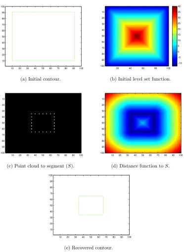
method of Zhao et al. [79]. This is demonstrated on a sparse 2D point cloud

in Figure 2.1, although the evolution equation used:

∂φ

∂t =∇d(x)· ∇φ+d(x)∇ ·

∇φ

|∇φ|, (2.19)

is different than the one used by Zhao et al. [79] in that it incorporates mean

curvature in the regularization.

2.7 Flux-based Functionals

Unlike Zhao et al. [79] who utilize distance from sparse surface points,

Savad-jiev et al. [62] reconstruct the surface by utilizing a field of vectors that are

normal to the surface. They assume that for the points in a small

neighbour-hood there exists a surface that the points have been sampled from. They

find normals and smooth them based on local curvature, and then solve for

the flux. Flux takes a vector field as input and produces a scalar which is

essentially the amount of flow through a unit area of a surface. A minimizer

for the functional

f lux(t) =

Z 1

0

< V, N >||Cp||dp=

Z L(t)

0

(32)

10 20 30 40 50 60 70 80 90 100 10 20 30 40 50 60 70 80 90 100

(a) Initial contour.

20 40 60 80 100

10 20 30 40 50 60 70 80 90 100 −10 −5 0 5 10 15 20 25 30 35 40

(b) Initial level set function.

10 20 30 40 50 60 70 80 90 100 10 20 30 40 50 60 70 80 90 100

(c) Point cloud to segment (S).

10 20 30 40 50 60 70 80 90 100 10 20 30 40 50 60 70 80 90 100

(d) Distance function toS.

10 20 30 40 50 60 70 80 90 100 10 20 30 40 50 60 70 80 90 100

(e) Recovered contour.

(33)

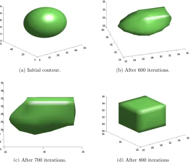
(a) Initial contour. (b) After 600 iterations.

(c) After 700 iterations. (d) After 800 iterations

(34)

is found using level sets as described in 2.2. The normal vector field of a

level set φ isN =δφ/|δφ|. The point cloud to which we wish to fit a surface

has normal information for each point, but a dense field is required to evolve

the level set. A box filter is used obtain F but propagate smoothed normal

information. F drives surface evolution towards the points

φt+F φ= 0. (2.21)

The idea of using flux for segmentation was introduced by Vasilevskiy and

Siddiqi [72] and applied to 2D and 3D MRA images of blood vessels. They

take an image I and compute the flux by using its gradient ∇I as the vector

field V, wishing to maximize the flux through its boundary, which is either a curve or a surface.

2.7.1 Continuous Global Optimization

Pan and Skala [52] start with a set of points with weak orientation data (like

[38]) and use total variation to measure the smoothness of function

Es =

Z Z Z

S

|∇f(x, y, z)|dxdydz (2.22)

where | · | is the L1 norm. A smaller norm indicates a more smooth function,

which a larger norm means the space is less smooth.

They use flux for their data term. A vector fieldF approximates the normal

directions via a smoothing filter. They designEdsuch that the gradient of the

implicit function is best aligned with this vector field

Ed=

Z

Ω

(35)

i.e. the optimal dot product between ∇f and F is zero.

2.7.2 Global Minimization for Shape Fitting

Lempitsky and Boykov [38] build on both graph cuts and Savadjiev et al.’s

[62] functional. They choose to solve for a sparse set of normals where only

weak orientation data is necessary. They too utilize a flux-based functional

max←−S

Z

S

< vs, ns > ds, (2.24)

though they solve for a thin band around the discretized points on the grid,

which is expanded as as needed using their TouchExpand [38] algorithm. Neighbouring nodes are connected via n-links, these represent the

regu-larizing term. The data term is represented by t-links, where nodes with

potentials greater than zero U(p)> 0 are connected to the source and nodes

with potentials less than zeroU(p)<0 are connected to the sink.

2.7.3 Power Watersheds

Couprie et al. [20] also use a graph based solution to find a solution to the

total variation problem mentioned above, specifically looking for the solution

u to

min

u∈[0,1] Z

Ω

w(z)p|∇u(z)|q_dz, _(2.25)

subject to u(z) = 0∀z ∈ Ωin and u(z) = 1∀z ∈ Ωout, where Ωin is the set

of labels inside of the surface and Ωout is the outside set. They construct a

graph G of edges (E) and nodes (V), discretizing the points on the grid and

(36)

Each unlabeled sub-graph with maximal weight is merged into a single

point, and then for each plateau (a maximal set of connected edges with

iden-tical weight), we look in the neighbourhood of each node and assign the node

the value

min

x

X

eij inE

w_ijp|xi−xj|q (2.26)

s.t.x(F) = 1, x(B) = 0. (2.27)

where

wij = min(dP(i), dP(j)),

and dP(·) is the distance between the nearest point in the set of all nodes P.

The power watersheds algorithm looks for a labeling xx of G, which is

initialized with seed labelsx(B) andx(F) on some points.

The algorithm is evaluated by iteratively finding an unlabeled node with

maximal weight, and then finding the maximal sub-graph of edges with equal

weight.

If this graph contains nodes with a known label then we find the surface

label based on minimizing Equation (2.26). Otherwise, all nodes are merged

and we find the next unlabeled node with maximal weight. Like Boykov and

Lempitsky [38], the power watershed algorithm can operate in a thin band,

which they define as the subset of the grid where the thresholded distance

(37)

2.8 Summary of Methods

The previous sections provided an overview of energy based methods for

sur-face fitting to point clouds. Some of the reviewed algorithms are in 2D space,

but the problems in 2D and 3D are extremely similar, and many of the 3D

algorithms described above were inspired by the 2D algorithms mentioned.

Graph cut based methods have proved to be extremely effective for 3D

surface fitting, as have TV methods. Surfaces constructed using graph cuts

will have small metrification artifacts [5], and level sets based methods will

often get stuck in local minima. TV methods lack metrification artifacts, but

are difficult to implement when compared with graph cuts. Both are great

(38)

Chapter 3 A Method for Quantitative

Comparison of 4D-CT Lung

Tumour Segmentations

3.1 Introduction

Internal imaging techniques have made it possible to develop treatments that

are minimally invasive. It is, however, incredibly difficult for an oncologist

to accurately determine the boundaries of a tumour; there is huge variability

among a group of oncologists’ segmentations of a tumour in a single patient.

Inter-observer variability is the biggest source of uncertainty in treatment

plan-ning in radiotherapy [31]. We wish to quantify treatment variability based on

target volume segmentation both prior to and following radiotherapy planning

stages. The gross tumour volume (GTV) is the portion of the tumour that can

be imaged: its volume does not necessarily contain the entirety of tumuorous

(39)

four-dimensional computed tomography (4D-CT) is complicated by tumour motion

during the breathing cycle. Oncologists therefore provide segmentations at ten

breathing phases (0%,10%,· · · ,90%) to ensure that dosages will be applied

to the entirety of the tumour. These respiratory phases each represent a

per-centage of full inspiration.

In addition, tumours are “gated”, which essentially means that some

ad-justment for the tumour’s position between these breathing phases is accounted

for using some type of motion tracking. Generating a 4D-CT usually involves

combining multiple 3D-CTs at various phases of the breathing cycle.

There has been substantial research into auto-segmentation of target

vol-umes from 4D-CT, but currently the most effective method is to segment the

gross tumour volume (GTV) on each CT data set (i.e. each respiratory phase),

which we then combine these to form a single integrated gross tumour volume

(IGTV). To account for low contrast and/or unseen areas of disease, the

mar-gin of this volume is expanded by 5-10mm. We refer to this larger volume as

the clinical target volume (CTV); it is the area that we wish to treat.

Finally, a similar and related term is the planned treatment volume (PTV).

The PTV’s purpose is to address the fact that uncertainties exist in both the

planning and delivery of radiographic treatment. The dose may be distributed

unevenly, and likewise, there areas of the body for which exposure to radiation

would have severe effects, and thus the PTV must factor these things in as

well. These are referred to as organs at risk (OR) [12].

The data we utilize are unorganized point clouds, segmented tumours from

CT data; it is not intensity data. We start with the points that each physician

specified as the boundaries on each slice in the CT data. The CT scans and

segmentations were obtained at the London Regional Cancer Program. The

(40)

contributors, and are present to help explain the larger significance of the

work.

We contribute a method for computing a similarity measure for the

volu-metric comparison of sparse point clouds of tumours as segmented from CT

data (as well as the actual computation of volumetric overlap and

distance-based error) for the compared point clouds in the data set.

3.2 Background

For reasons we described in Chapter 2, we rely on Lempitsky and Boykov’s

[38] flux-based method for providing a globally optimal surface for each point

cloud. Their method solves for a sparse set of normals where only weak

ori-entation data is necessary. They rasterize the points onto a dense 3D volume

and solve their functional on a thin band surrounding the points, using the

Touch Expand algorithm. Touch Expand is an algorithm for solving max-flow

problems on a graph with source and sink arcs.

The surface fitting function

max←−S

Z

S

< vs, ns> ds (3.1)

uses normals and the surface velocity and is specifically for the circumstance

when perfect data is available. That is obviously not the case here, and thus

the elastic membrane prior is utilized. We want to compute

min←−S

Z

S

λds−

Z

S

< v, ns> ds. (3.2)

(41)

s and the sink t. We then have non-terminal nodes p ∈ P, each of which represents a voxel and is connected to its neighbouring nodes via n-links and

terminal links of the form (s, p) and (p, t), as was explained in Section 2.3.

Neighbouring nodes are connected via n-links, these represent the

regu-larizing term. The data term is represented by t-links, where nodes with

potentials greater than zero U(p)> 0 are connected to the source and nodes

with potentials less than zeroU(p)<0 are connected to the sink.

We also utilize the method’s closed topology, which works by extending

the boundary of the dense grid in each dimension and setting the boundary

points’ t-links to a large, negative value.

The sparse vector field {¯vi|p¯i ∈ P} is blurred by the width of the flux’s

diffuse radius, a parameter set prior to run-time. In practice, a box filter is

used to perform thisntimes, wheren is a preset parameter. The result of this

blurring is to obtain a semi-dense field ¯vp = ΣNi=1¯vpi. These vectors are a set

of semi-dense averaged normals, obtained by applying said box filter to sparse

normals.

3.3 Problem

The method by which physicians segment a dense 4d image to produce a 3D

point cloud, outlining the perimeter of 2D slices, produces a set of points that

incompletely describes the surface. Specifically, the segmentation is performed

by a physician in an application called Pinnacle Treatment Planning System

[67]. On the periphery of each dimension, the edge is implied, i.e., in one

slice there will be a segmentation performed, and then in the adjacent slice

there won’t be. In some cases, the segmentation in the next-to-last slice will

(42)

current process of segmentation, not a problem with a physician failing to do

their job.

Given sparse and incomplete data, as we see on the top of Figure 3.1a, how

do we compare the difference between two point clouds in a meaningful way?

This makes using volumetric methods for comparison difficult. Similarly, using

point based methods don’t solve this problem either; we have large swaths

which are implied parts of the tumour that also need to be quantified.

3.4 Methodology

Ten patients with Non-Small Cell Lung Cancer (NSCLC) were imaged

us-ing 4d-CT usus-ing a Big Bore CT scanner, along with the Real-time Position

Management (RPM) system for gating. The 4d data has x, y, z and intensity

values, where thez-axis is the coronal plane, the x-axis is the sagittal plane,

the y-axis is the axial plane and their units are in millimetres (mm). RPM

in-volves having markers placed on the patient’s abdomen or chest, and tracking

these markers using an infrared camera. Using this, the images are generated

at the breathing phases and correspond to one another, both for a patient’s

images captured at different phases, and other patients’ images captured at

the same phase [46].

Thus, 10 4D-CT images are generated for each patient, an example of

which can be seen in Figure 3.2 A 4D-CT can be thought of as a “stack”

of intensity images: a loaf of multi-coloured bread is an apt comparison. A

physician takes each of these “slices” for a single breathing phase, and must

identify the interior of the tumour for this slice from the exterior, typically

with a mouse by clicking around the boundary of the tumour. In addition

(43)

(a)

(b)

(44)

(45)

is inter-observer variation [31] – it is also a highly time consuming task, as a

single 4D-CT image often has more than 100 slices.

3.5 Point Cloud Construction

Each 2D point (xi, yi) is combined with itszs, the height (i.e. slice)

measure-ment, and these points are collected to make a single point cloud, an example

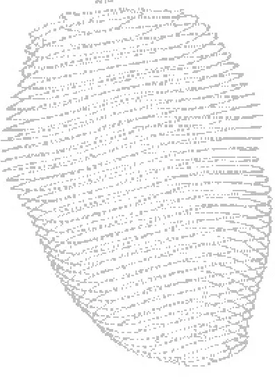
of which is seen in Figure 3.3. The larger goal of this work is to determine the

efficacy of treatment, but the technical goal is to deliver a method that can

consistently measure how well the treatment is administered, i.e. how much

overlap there is between the tumour and the treated area.

(46)

3.5.1 Surface Fitting

The nature of the point clouds combined with our need for a watertight surface

created a significant challenge in providing an accurate surface fitting. If one

thinks about the slices of a 3D-CT, the “top” of the tumour will typically be

quite wide in terms of the segmentation. The other points are generally fairly

evenly-spaced, but the top and bottom often have a large gap and this makes

getting a “tight” fitting surface a problem. To generate accurate, automated

and watertight segmentations for almost 1000 images is a challenge.

The flux based surface fitting method requires approximate orientation

data for computing the max-flow/min-cut. It is, as they note, acceptable to

use a single normal for all points in a single range scan. We do not have the

benefit of such orientation information, so we first fit an approximate surface

and then find vertex normals based on this surface.

Our C++ application (trimesh normal) that imported each of these files sequentially first constructed an approximate surface mesh to get a field of

normal vectors that is approximates the true field. We used the ball pivoting

algorithm to first fit the approximate surface, and then compute the normals

using said surface. Our application uses VCGLIB’s [18] routines for ball

pivot-ing, normal estimation and orientation, and TouchExpand [38] for watertight

surface fitting.

Ball pivoting is an advancing front algorithm [1]. A “seed” point is selected,

and two neighbours are searched for such that they can be circumscribed in the

radius of the ball with an empty interior. If such a pair of vertices are found,

a triangle is created [22]. The ball is then pivoted, i.e. it is rotated around the

edge until it circumscribes another point, forming another triangle. In the case

(47)

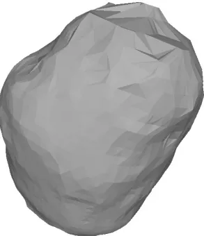
Figure 3.4: Approximate meshed surface for point cloud seen in Figure 3.3, as fitted using the ball pivoting algorithm.

edge is chosen. This process is continued until all edges have been traversed,

at which point a new seed triangle is found [1].

The ball pivoting algorithm is uses a sphere of radius r (in our caser = 1)

and “rolls” it over the point cloud, adding a triangle (i.e. edges and a surface)

if the ball contains three points only. In Figure 3.4 we see the approximate

sur-face fit after ball pivoting has been applied, which we then utilize to compute

(48)

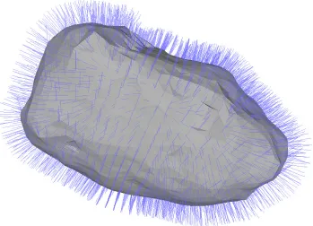
Figure 3.5: Normals calculated for an approximate surface.

3.5.2 Computing Normals

We first calculate the per face normals for our newly-constructed mesh. For

each triangle with vertices p1, p2, p3, we calculate vector u = p1 − p2 and

v = p3 −p1, then the normal n = u×v. The choice of variable assignment

determines the orientation of the normal, i.e., whether it points inward or

outward, so we wind the normals subsequently.

We then normalize the lengths of these normals and utilize them to compute

the normal for each vertex. We use equally weighted averaging of facets, i.e.

nv||

P3

i=1ni, where nv is a vertex normal and || implies parallelism and thus

subsequent normalization, i.e. nv =nv_|n_nv_v_|, we borrow this notation from [35].

As we said above, the computed normals’ orientation is strictly based on

(49)

they are pointing outward, an example of such a field can be seen in Figure

3.5.

Computing accurate surfaces for each patient ended up being heavily

com-putationally expensive. Computing almost 1000 watertight, globally optimal

surfaces is expensive, and one of our requirements was that the resultant 3D

volumes are comparable. Our bounding box encapsulated every point, but

also had a boundary at the maximum and minimum of each dimension, as

TouchExpand needs sufficient space around a voxel to approximate the energy

using neighbouring voxels: when neighbouring points are boundaries, we

expe-rienced trouble with convergence. We settled on a grid size of 150×150×150,

which is quite large and resulted in expensive surface computations, but given

that the bounding box encapsulatedalltumours, it was necessary to have high resolution since in practice some tumour volumes would only be occupying a

small amount of the bounding box.

There was an element of trial and error in generating a set of terms that

could accurately capture an appropriate surface for our entire set of point

clouds. In practice it was very easy to tell when a surface was not watertight:

when we computed the volumetric overlap [28] whereEo is zero when overlap

is perfect, and one when no overlap exists.

3.5.3 Minimal Surface Fitting to Segmented Point Cloud

As we discussed in Chapter 2, we use the minimal surface as a guiding principle

for our surface fitting: we wish to obtain the surface with a volume that

encapsulates the points to which we are trying to fit the surface. In the

preliminaries, we mentioned that this idea was introduced to the vision world

(50)

minima due to the level sets implementation.

Instead, we use a graph cuts-based method, specifically the flux-based

method as introduced by Boykov and Lempitsky [38]. Again, as we

men-tioned in the introduction, graph cuts-based methods promise to provide a

global minimizer for the proposed functional.

From the ball pivoting algorithm, we now have a mesh, comprised of faces

with normals, from which we generate vertex normals. We then rasterize our

vertices onto a discrete grid and compute the flux for these points.

For our purposes, we used TouchExpand with a topology constraint (closed

surface) with a larger diffuse radius for the flux (df = 2, versus the default of

df = 1), as well as an extra iteration. This is to ensure that we can guarantee

a closed surface.

The result of TouchExpand is a binary, dense 3D volume where the inside

of the point cloud is marked by 1’s and the outside by 0’s. Given our problem

of computing volumetric overlap, this is convenient, as we can compute Eo

directly by just iterating over all points.

We performed a cursory visual inspection of each generated mesh to

en-sure a watertight result, however, our method could easily detect when we

lacked convergence, i.e. a closed surface. If the volumetric overlap was less

than a reasonable threshold (generally 70%), it was usually obvious that

trimesh normal surfhad failed to obtain a watertight surface for one (or both) of the point clouds. While each tumour had been segmented by eight doctors,

(51)

3.6 Similarity Quantification

We chose the method of Lempitsky and Boykov [38] after our evaluation of

many methods, as seen in Chapter 2, primarily because it solves both our core

problems. Surface evolution methods and local methods cannot guarantee

finding a global minimum when fitting a watertight surface to a point cloud.

Their TouchExpand library is freely available and has an optional shape prior

for closed surfaces.

Definition 3.6.1 (Volumetric Overlap). For two watertight surfacesS andG

that exist on the same grid structure, if all occupied voxelssi are occupied by

Gand all voxelsgi are occupied byS, we say that a perfect volumetric overlap

(V OE = 0) occurs

More specifically, the volumetric overlap is

Eo(S, G) = 1−(|S∩G|)/(|S∪G|). (3.3)

We use Eo, a.k.a. the Jaccard index because, as we point out in [46],

usingR2 error is disproportionately punishing as distance increases between a source and target. Moreover, the numbers aren’t comparable between tumours

of largely varying sizes: we wish to know how well the physician performed

independent of the size of the tumour.

Definition 3.6.2 (Nearest Neighbour of xand Y). For a pointx, the nearest

neighbour in a set of points Y = {y1,· · · , yn} is the point yi with minimum

Euclidean distance from x, i.e.

N N(x, Y) = minp(x−yi)2,∀yi ∈Y .

(52)

Definition 3.6.3 (Nearest Neighbours of X and Y). For a set of points X,

the nearest neighbours of a set of points Y is a set such that N N(X, Y) =

N N(xj, Y)∀xj ∈X .

Definition 3.6.4 (Symmetric Nearest Neighbour). For two sets of points X

and Y, two pointsxm and yn are considered symmetric (i.e. mutual) nearest

neighbours ifynis the nearest neighbour ofxm andynis the nearest neighbour

of xm.

In practice, we store our point clouds in kdtrees to improve the complexity

of computing nearest neighbour options, which we use to compute the

sym-metric RM S−E, which is the RM S−E for symmetric nearest neighbours.

3.7 Results

As we see in Figure 3.10, segmentations of patient B’s GTV will vary greatly

among physicians. Each colour represents a different physician’s segmentation.

In the top left and bottom left of Figure 3.10, we see a large difference on

the y-axis; each physician has a very different view of what does and does not

encompass the tumour. Indeed, the reconstructions shown in the bottom right

of Figure 3.10 (each has a different colour), are extremely different from one

another.

This, in fact, is a moderate variation. Figures 3.6 and 3.7 show how

dra-matically different a set of physicians’ interpretation of what does and does

not constitute a tumour can be in both primary and nodal data.

For the VOE of the primary IGTV, the combined GTVs from all 10

breath-ing phases, in terms of observer (intra-patient) we saw a large variation.

(53)

(a)

(b)

(c)

(54)

(a) (b)

(c) (d)

(e) (f)

(55)

Figure 3.8: Graph of volumetric overlap for gated tumours for each patient.

(56)

(9.0± .6) to (35.6±7.5) and in nodal tumours (16.4±.5) to (29.1±4.1).

We saw inter-patient σ from 0.6% to 13.2% for primary tumours and from

1.5% to 13.1% for nodal tumours. For symmetric RMS distances

(individ-ual results can be seen in Figure 3.9), we saw (3.4±.4)mm to (7.8±.8)mm

for primary IGTVs with standard deviations in the range (0.2mm,1.2mm).

The nodal IGTVs had mean observer RMS symmetric distances ranging from

(4.1±.8)mm to (6.5±.7)mm with σ ranging from 0.2mm to 3.2mm. Note

that RMS is a distance but VOE is a ratio, hence the lack of a unit in the

former.

The symmetric RMS distances are affected by the size of the tumour

vol-ume, and the nodes are smaller than the primary volume. It is also

substan-tially more difficult to accurately segment the nodal volumes, parsubstan-tially because

nodes tend to exist in low contrast areas.

Both lymph nodes can be affected, in which case there will be more than

one nodal volume. The process of constructing an initial, approximate

sur-face, calculating surface normals and then utilizing [38] handles this constraint

effectively, utilizing the same parameters as those used for the GTV to ensure

that comparisons are fair.

For each of the hundreds of segmented point clouds, our method

success-fully fit a watertight figure, some examples of which can be seen in Figures 3.1.

This required an element of trial and error, as it was necessary to find

param-eters that would avoid smoothing out contours and still maintain a watertight

surface. Our results demonstrate a clear trend, so in addition to guarantees

that TouchExpand provides in terms of optimality, we can feel confident that

it successfully captures an accurately modeled, representative shape.

The COVs (coefficient of variation) of physician segmentations of both the

(57)

Table 3.1: Coefficient of Variation for VOE.

Two patients did not have nodal tumours, but of the five of the eight who did,

the COVs of nodal IGTVs were larger than the primary IGTVs, though for

patient D, the primary GTV has a very large COV (93.25%). Overall, both

nodal and primary GTV segmentations tend to have very high COVs.

3.8 Conclusions and Future Work

One clear conclusion from our research is that there is a high degree of variation

among physicians’ interpretations of what is and is not tumourous growth and

thus their resultant segmentations and dose distributions are highly variable.

This is true of both primary and nodal tumours, and though nodal tumour

performance is more variable, both suffer from the same problem to a large

degree.

Advancements in technology have brought about improved target

localiza-tion via gating of imaged data, as well as methods to more effectively target

tumours with radiation. The process of segmentation remains error prone;

(58)

performance of physicians and help ensure that patients are being given

ap-propriate dosages.

Because the human cost is so high, experimentation is limited. The data set

that we have produced here was hugely time consuming to compile, meanwhile,

limited human and physical capital within the health-care system is the norm.

Any steps toward automation and standardization will be a huge win, and the

method presented is a step in that direction.

We would like, in future work, to perform a similar analysis on different

types of tumours, in hopes of obtaining a quantitative measure of what types

(59)

(60)

Chapter 4 Global Registration of Multiple

Thin Structures

Building a 3D model is extremely useful for many practical applications where

inferring measurements about the shape or size of an object is a

require-ment. With the rapid acceleration of hardware capability in terms of CPU

power, storage and 3D scanners, we can now capture huge amounts of data

and the fidelity of the resultant models is constrained by the quality of

merg-ing/reconstruction algorithms. Due to recent advancements of robotic

tech-nologies and low cost laser scanners, building real time automated systems

is becoming possible for plant science and agricultural applications, where a

major task is to build a 3D model of the plant to analyze different biological

properties (like growth, etc.). However, the complex recursive structure of

a plant makes the problem of aligning multiple views extremely hard, unlike

building a 3D model of a rigid object like Stanford bunny. Also in medical

robotics, automatic analysis of medical images is a crucial step. A common