Scholarship@Western
Scholarship@Western
Electronic Thesis and Dissertation Repository
4-24-2018 11:30 AM
Putting Fürer's Algorithm into Practice with the BPAS Library
Putting Fürer's Algorithm into Practice with the BPAS Library
Linxiao Wang
The University of Western Ontario
Supervisor
Moreno Maza, Marc
The University of Western Ontario
Graduate Program in Computer Science
A thesis submitted in partial fulfillment of the requirements for the degree in Master of Science © Linxiao Wang 2018
Follow this and additional works at: https://ir.lib.uwo.ca/etd
Part of the Algebra Commons, and the Other Computer Sciences Commons
Recommended Citation Recommended Citation
Wang, Linxiao, "Putting Fürer's Algorithm into Practice with the BPAS Library" (2018). Electronic Thesis and Dissertation Repository. 5358.
https://ir.lib.uwo.ca/etd/5358
This Dissertation/Thesis is brought to you for free and open access by Scholarship@Western. It has been accepted for inclusion in Electronic Thesis and Dissertation Repository by an authorized administrator of
Abstract
Fast algorithms for integer and polynomial multiplication play an important role in scientific computing as well as other disciplines. In 1971, Sch¨onhage and Strassen designed an algorithm that improved the multiplication time for two integers of at most n bits toO(lognlog logn). In 2007, Martin F¨urer presented a new algorithm that runs inOnlogn ·2O(log∗
n), where log∗ n is the iterated logarithm ofn.
We explain how we can put F¨urer’s ideas into practice for multiplying polynomials over a prime fieldZ/pZ, which characteristic is a Generalized Fermat prime of the form p = rk +1 wherekis a power of 2 andris of machine word size. Whenkis at least 8, we show that mul-tiplication inside such a prime field can be efficiently implemented via Fast Fourier Transform (FFT). Taking advantage of Cooley-Tukey tensor formula and the fact thatris a 2k-th primitive root of unity, we obtain an efficient implementation of FFT over Z/pZ. This implementation outperforms comparable implementations either using other encodings ofZ/pZor other ways to perform multiplication inZ/pZ.
Keywords: F¨urer’s algorithm, Fast Fourier Transform, Generalized Fermat prime, polyno-mial multiplication
Abstract i
List of Algorithms iv
List of Code Listings v
List of Figures vi
List of Tables vii
List of Appendices viii
1 Introduction 1
1.1 F¨urer’s trick . . . 2
1.2 Thesis organization and contributions . . . 3
2 Background 5 2.1 Prime field arithmetic . . . 5
2.1.1 Primitive root of unity . . . 6
2.1.2 Montgomery multiplication . . . 7
2.2 The discrete Fourier transform and the fast Fourier Transform . . . 8
2.3 Multiplication time . . . 10
2.4 Dense univariate polynomial multiplication . . . 10
2.5 BigOandΘnotations . . . 13
2.6 Syntax of pseudo-code . . . 14
3 Generalized Fermat prime field arithmetic 15 3.1 Representation ofZ/pZ . . . 16
3.2 Computing the primitive root of unity inZ/pZ . . . 16
3.3 Addition and subtraction inZ/pZ . . . 17
3.4 Multiplication by power ofrinZ/pZ . . . 19
3.5 Multiplication between arbitrary elements inZ/pZ . . . 20
4 Optimizing multiplication in Generalized Fermat prime fields 22 4.1 Algorithms . . . 22
4.1.1 Based on polynomial multiplication . . . 22
4.1.2 Based on integer multiplication . . . 26
4.2 Analysis . . . 26
4.2.1 Based on polynomial multiplication . . . 27
4.2.2 Based on reduction to integer multiplication . . . 28
4.3 Implementation with C code . . . 29
5 A generic implementation of FFT over finite fields in the BPAS library 37 5.1 The tensor algebra formulation of FFT . . . 37
5.2 Finite fields in the BPAS library . . . 39
5.3 BPAS implementation of the FFT . . . 41
6 Experimentation 46 6.1 FFT over small prime fields . . . 46
6.2 Multiplication in generalized Fermat prime fields . . . 48
6.3 FFT over big prime fields . . . 50
7 Conclusion 53
Bibliography 54
A C Functions for Multiplication in Generalized Fermat Prime Field 56
Curriculum Vitae 63
2.1 Computing then-th primitive root of unity overGF(p) . . . 7
2.2 The Fast Fourier Transform . . . 9
2.3 Karatsuba Multiplication . . . 11
2.4 Fast Convolution . . . 12
3.1 PrimitiveN-th rootω∈Z/pZsuch thatωN/2k =r . . . 17
3.2 Computingx+y∈Z/pZforx,y∈Z/pZ . . . 18
3.3 Computingx·y∈Z/pZforx,y∈Z/pZ . . . 21
4.1 An algorithm for rewritingxiyjintol+hr+cr2 . . . 25
4.2 Computingu=x y∈Z/pZforx,y∈Z/pZusing polynomial multiplication. . . 26
4.3 Computingx y∈Z/pZforx,y∈Z/pZusing integer multiplication . . . 26
4.4 Computing fx(R)· fy(R) mod (Rk+1) inZ/qZusing Negacyclic Convolution . . . . 30
4.5 Chinese Remainder Algorithm computing equation 4.18 . . . 33
4.6 Computings1264+s0 =l+h r+c r2 . . . 34
4.7 FFT-based multiplication for two arbitrary elements inZ/pZ . . . 35
4.8 Montgomery Multiplication inZ/qZ . . . 36
5.1 Computing DFT onKepoints inZ/pZ . . . 42
5.2 Unrolled DFT base-case whenK=8 . . . 45
List of Source Code Listing
3.1 Addition in a Generalized Fermat Prime Field . . . 18
3.2 Multiplication by power if r in a Generalized Fermat Prime Field . . . 20
4.1 Modular funtion using reciprocal division . . . 32
4.2 Multiplication between two 64-bit numbers . . . 32
5.1 Calling sequence ofSmallPrimeFieldclass in the BPAS library . . . 40
5.2 Calling sequence ofSmallPrimeFieldmacro in the BPAS library . . . 41
5.3 Stride permutation for FFT . . . 42
5.4 Twiddle factor multiplication for FFT . . . 43
A.1 Multiplication between two 128-bit numbers . . . 56
A.2 Chinese Remainder Algorithm . . . 57
A.3 Computing the quotient and remainder of a machine word size number divided by a radix r . . . 59
A.4 (l,h,c) Algorithm . . . 60
A.5 Montgomery multiplication for 64-bit numbers . . . 62
2.1 FFT-based univariate polynomial multiplication . . . 13
6.1 FFT over small prime field withDFT8 . . . 47
6.2 FFT over small prime field withDFT16 . . . 47
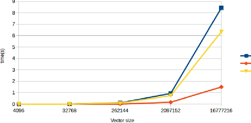
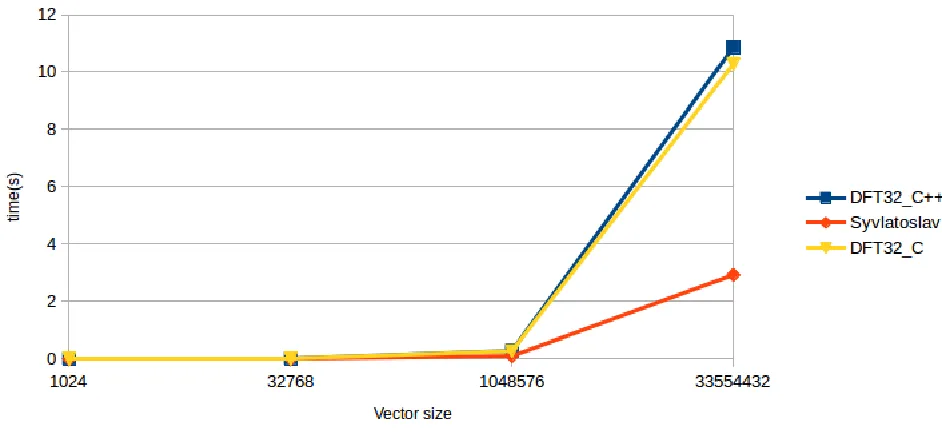
6.3 FFT over small prime field withDFT32 . . . 48
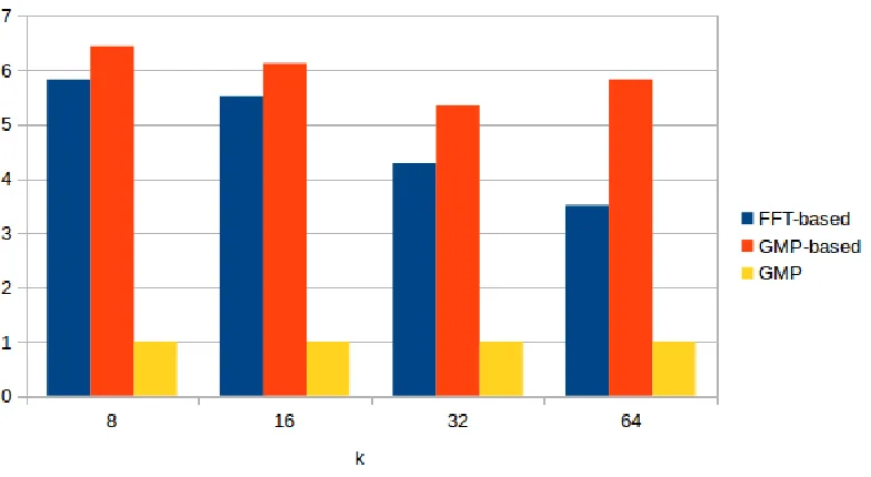
6.4 FFT-based multiplication vs. GMP-based multiplication vs. GMP multiplication . . . 49
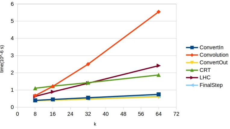
6.5 Time spends in different parts of the FFT-based multiplication . . . 50
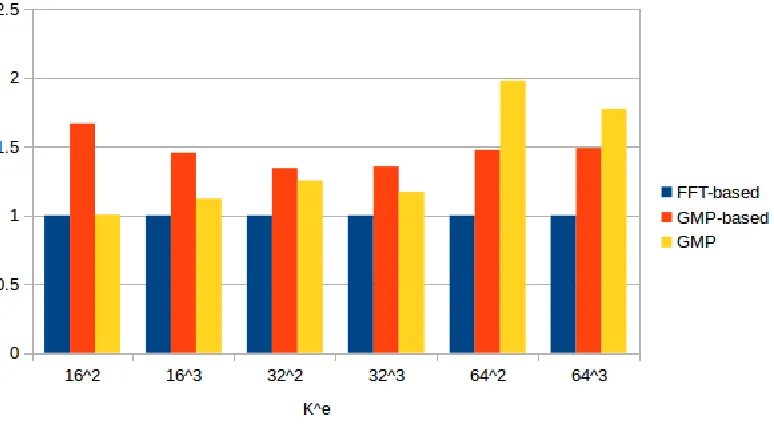
6.6 FFT of sizeKe whereK=16 . . . 51
6.7 Average time of one multiplication operation in FFT . . . 52
List of Tables
2.1 Multiplication time of different algorithms.. . . 13
3.1 SRGFNs of practical interest. . . 16
5.1 Numbers of lines in n-point unrolled FFT. . . 45
6.1 Time cost of one multiplication operation using FFT-based, GMP-based and GMP approaches. . . 49
6.2 Time cost in different parts of the FFT-based multiplication in percentage.. . . 50
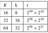
6.3 Primes used for different base-cases . . . 51
6.4 Time cost of FFT on vector sizeKeover different prime fields . . . 51
6.5 Time spend in different parts of the FFT function whenK=64,e=3 . . . 52
6.6 Average multiplication time of FFT over big prime fields (Time is in ms) . . . 52
Appendix A . . . 56
Chapter 1
Introduction
Asymptotically fast algorithms for exact polynomial and matrix arithmetic play a central role in scientific computing. Among others, the discoveries of Karatsuba [21], Cooley and Tukey [6], Strassen [27], and Sch¨onhage and Strassen [25] have initiated an intense activity in both numer-ical computing and symbolic computation. The implementation of asymptotnumer-ically fast algo-rithms is, on its own, a research direction. Often the theoretical analysis of asymptotically fast algorithms focuses on arithmetic operation counts, thus ignoring important hardware details, in particular costs of memory accesses. On modern hardware architectures, these theoretical sim-plifications are questionable and other complexity measures, such as cache complexity [14], are needed to better analyze algorithms.
In the past two decades, several software for performing symbolic computations have put a great deal of effort in providing outstanding performance, including successful implemen-tation of asymptotically fast arithmetic. As a result, the general-purpose computer algebra system Magma[5] and the Number Theory Library NTL [26] have set world records for poly-nomial factorization and determining orders of elliptic curves. The book Modern Computer Algebra[17] has also contributed to increase the general interest of the computer algebra com-munity for these algorithms. As for linear algebra, in addition to Magma, let us mention the C++template library LinBox [20] for exact, high-performance linear algebra computation with dense, sparse, and structured matrices over the integers and over finite fields. A cornerstone of this library is the use of BLAS libraries such as ATLAS to provide high-speed routines for matrices over small finite fields, through floating-point computations [11].
The algorithm of Sch¨onhage and Strassen [25] is an asymptotically fast algorithm for mul-tiplying integers in arbitrary precision. It uses the fast Fourier transform (FFT) and, for two integers of at mostnbits, it computes their product inO(nlogn·log logn) bit operations. This result remained the best known upper bound until the celebrated paper of Martin F¨urer [15]. His integer multiplication algorithm runs in Onlogn ·2O(log∗n) bit operations, where log∗
n is the iterated logarithm ofn, defined as:
log∗n:=
0 ifn≤1;
1+log∗(logn) ifn>1 (1.1)
A detailed analysis suggests that F¨urer’s algorithm is expected to outperform that of Sch¨onhage and Strassen forn≥2264.
The practicality of F¨urer’s algorithm is an open question. And, in fact, the work reported in this thesis is a contribution responding to this open question. Before presenting our approach, we observe that the ideas of F¨urer are not specific to integer multiplication and can be used for multiplying polynomials with coefficients in the field of complex numbers or in a finite field. In [9, 10] Anindya De, Piyush P. Kurur, Chandan Saha and Ramprasad Saptharishi gave a similar algorithm which relies onfinite field arithmetic and achieves the same running time as F¨urer’s algorithm. Working with polynomials with coefficients in a finite field will be our framework. Hereafter, we explain the “main trick” of F¨urer’s algorithm. To this end, we follow an analysis reported by Liangyu Chen, Svyatoslav Covanov, Davood Mohajerani and Marc Moreno Maza in [4].
1.1
F ¨
urer’s trick
Consider a prime fieldZ/pZandN, a power of 2, dividing p−1. Then, the finite fieldZ/pZ admits anN-th primitive root of unity1. Denote such an element byω. Let f ∈ Z/pZ[x] be a polynomial of degree at mostN−1. Then, computing the DFT of f atωvia an FFT produces the values of f at the successively powers of ω, that is, f(ω0), f(ω1), . . .f(ωN−1). Using an asymptotically fast algorithm, namely a fast Fourier transform (FFT), this calculation amounts to:
1. N log(N) additions inZ/pZ,
2. (N/2) log(N) multiplications by a power ofωinZ/pZ. If the size of piskmachine words, then
1. each addition inZ/pZcostsO(k) machine-word operations,
2. each multiplication by a power ofωcostsO(M(k)) machine-word operations,
wheren 7−→ M(n) is a multiplication time as defined in Section 2.3 Therefore, multiplication by a power ofωbecomes a bottleneck askgrows. To overcome this difficulty, we consider the following trick proposed by Martin F¨urer in [15, 16]. We assume that N = Ke holds for some
“small” K, say K = 32 and an integere ≥ 2. Further, we define η = ωN/K, with J = Ke−1 and assume that multiplying an arbitrary element of Z/pZ by ηi, for any i = 0, . . . ,K − 1,
can be done withinO(k) machine-word operations. Consequently, every arithmetic operation (addition, multiplication) involved in a DFT onK points, usingηas a primitive root, amounts to O(k) machine-word operations. Therefore, such DFT of size K can be performed with O(K log(K)k) machine-word operations. instead ofO(K log(K)M(k)) without the assumption. Since the multiplication time n 7−→ M(n) is necessarily super-linear, the former estimate is asymptotically smaller than the latter one. As we shall see in Chapter 3, this result holds whenever pis a so calledgeneralized Fermat number.
Returning to the DFT of size N at ω and using the factorization formula of Cooley and Tukey [6], we have
DFTJK = (DFTJ ⊗IK)DJ,K(IJ⊗DFTK)LJKJ , (1.2)
see Section 5.1. Hence, the DFT of f atωis essentially performed by:
1.2. Thesis organization and contributions 3
3. K DFT’s of sizeKe−1.
Unrolling Formula (1.2) so as to replace DFTJby DFTKand the other linear operators involved
(the diagonal matrixDand the permutation matrix L) one can see that a DFT of sizeN = Ke
reduces to:
1. e Ke−1DFT’s of sizeK, and
2. (e−1)Nmultiplications by a power ofω.
Recall that the assumption on the cost of a multiplication byηi, for 0 ≤ i< K, makes the cost for one DFT of size K toO(K log2(K)k) machine-word operations. Hence, all the DFT’s of sizeKtogether amount toO(e N log2(K)k) machine-word operations. That is,O(N log2(N)k) machine-word operations. Meanwhile, the total cost of the multiplication by a power ofω is O(e NM(k)) machine-word operations, that is,O(N logK(N)M(k)) machine-word operations.
Indeed, multiplying an arbitrary element ofZ/pZby an arbitrary power ofωrequiresO(M(k)) machine-word operations. Therefore, under our assumption, a DFT of sizeNatωamounts to
O(N log2(N)k + N logK(N)M(k)) (1.3)
machine-word operations. When using generalized Fermat primes, we have K = 2k and the
above estimate becomes
O(N log2(N)k + N logk(N)M(k)). (1.4)
The second term in the big-O notation dominates the first one. Without our assumption, as discussed earlier, the same DFT would run in O(N log2(N)M(k)) machine-word operations. Therefore, using generalized Fermat primes brings a speedup factor of log(K) w.r.t. the direct approach using arbitrary prime numbers.
In this thesis, we are addressing two questions. First, can we observe this speedup fac-tor on a serial implementation written in the programming language C and run on modern multicore processors. Indeed, the authors of [4] answered a similar question in the case of a CUDA implementation targeting GPUs (Graphics Processing Units). Such architectures offer to programmers a finer control of hardware resources than multicore processors, thus more opportunities to reach high performance. Hence, this first question is a natural challenge.
Second, can we use FFT to implement multiplication in Z/pZ and obtain better perfor-mance than using plain multiplication inZ/pZ? This was not attempted in the GPU implemen-tation of [4]. However this is a natural question in the spirit of the algorithms of Sch¨onhage and Strassen [25] and F¨urer [15], where fast multiplication is achieved by “composing” FFTs operating on different vector sizes. The experimental results reported in Section 6 give positive answers to both questions.
1.2
Thesis organization and contributions
This thesis is organized as follows. Chapter 2 is a brief review of the concepts of a prime fieldand a multiplication time, the discrete Fourier transform, the fast Fourier Transform and its application to polynomial multiplication. Chapter 3 presents our implementation of prime fields of the formZ/pZwhere pis a Generalized Fermat prime number; this is based on and extends the work reported in [4].
Consider a Generalized Fermat prime number of the form p=rk+1, wherekis a power of 2
rmodulopcan be done inO(k) machine-word operations. However, multiplying two arbitrary elements ofZ/pZis a non-trivial operation. Note that we encode elements ofZ/pZin radixr expansion. Thus, multiplying two arbitrary elements ofZ/pZrequires to compute the product of two univariate polynomials inZ[X], of degree less thank, moduloXk+1. In [4], this is done by using plain multiplication, thusΘ(k2) machine-word operations. In Chapter 4, we explain how to multiply two arbitrary elements x,y ofZ/pZ via FFT. We give a detailed analysis of the algebraic complexity of our procedure. A natural alternative to our approach would be to compute (xy) mod pwhere the productxyis an integer computed after converting the radixr expansion of x,yto integers (say in binary expansions). We show that this alternative approach is theoretically and practically less efficient than the one via FFT.
In order to verify experimentally the benefits of F¨urer’s trick, we need to perform FFT computations over a Generalized Fermat prime field Z/pZ, for different implementations of that prime field. One should be able to assume that the elements of Z/pZ are in radix r ex-pansion (when p writesrk +1 where k is a power of 2) or one should simply be able to use traditional radix 2 expansions. Moreover, we consider multiplying two arbitrary elements of Z/pZ via FFT. Overall, we need an implementation of FFT running over a variety of prime fields. Chapter 5 reports on a generic implementation of FFT over finite fields in the BPAS library [3]. This part is a joint work with Colin Costello and Davood Mohajerani.
Chapter 2
Background
2.1
Prime field arithmetic
Arithmetic operations for polynomials and matrices over prime fields play a central role in computer algebra. It supports the computation over Galois fields that are essential to cryptog-raphy algorithms as well as coding theory. In symbolic computation, the implementation of the so-called modular methods, prime fields are often using machine word size characteristic. In-creasing the arithmetic to greater precision can be done using the Chinese Remainder Theorem (CRT).
However, using these small prime numbers can cause problems in some certain modular methods. In particular, the so-called unlucky primes are to be avoided [1, 8]. Because of the limitation of using small prime numbers, arithmetic over prime fields, where the primes are multi-precision numbers, is desired for some problems, for instance, polynomial system solving.
In algebra, a non-empty setAis aringwheneverAis endowed with two binary operations denoted additively and multiplicatively such that
• both addition and multiplication are associative,
• both addition and multiplication admit a neutral element, denoted respectively 0 and 1,
• addition must be commutative and every x ∈ A admits a symmetric element w.r.t. the addition, denoted−x.
• the multiplication is distributive w.r.t. the addition.
The ringAis commutativeif its multiplication is commutative. The commutative ringAis a field if every non-zerox∈Aadmits a symmetric element w.r.t. the multiplication, denotedx−1. Examples of fields are the setQof rational numbers, the setAof real numbers and the setCof complex numbers. Examples of rings that are not fields are the setZof integer numbers, the set of 2×2 matrices with coefficients inRand the set of univariate polynomials with coefficients inQ.
AGalois field, also known asfinite field, is a field with finitely many elements. The residue classes modulo p, where pis a prime number, form a field (unique up to isomorphism) called theprime field with p elements and denoted byGF(p) or Z/pZ. Single-precision and multi-precision primes are referred to assmall primesandbig primesrespectively.
Leta,bbe integers and pa prime number. The residue class ofainGF(p) is denoted bya
mod p. The sum and the product ofa mod pandb mod pare given by (a+b) mod pand a·b mod p, respectively. Ifb mod pis not zero, then the quotient ofa mod pbyb mod p is given bya·b−1 mod p, whereb−1 mod pis the inverse ofbinGF(p). The elementb−1 mod pcan be computed in different ways, for instance via the Extended Euclidean Algorithm,
see Chapter 5 in [17]. The maps (a,b,p) 7−→ a + b mod p, (a,b,p) 7−→ a· b mod p
and (a,b,p) 7−→ ab−1 mod pare often calledmodular addition,modular multiplicationand modular division.
2.1.1
Primitive root of unity
Primitive roots of unity are a special kind of elements in a field that are used by some algo-rithms, such as Fast Fourier transforms. For a fieldFand an integern≥1, an elementω∈Fis ann-th primitive root of unity, if it meets the following two requirements [17].
(i) ωis ann-th root of unity, that is, we haveωn= 1.
(ii) we haveωi , 1 for all 1<i< n.
This definition generalizes to the case whereFis a commutative ring by adjusting the second requirement as follows: for all 1< i<n, the elementωi−1 is not a zero-divisor.
It follows from a classical result in group theory, see [17], that the fieldGF(p) admits an n-th primitive root of unity if and only n divides p−1. Assume from now on that that this latter condition holds. Then, we can derive a simple probabilistic algorithm to compute ann-th primitive root of unity inGF(p). By assumption, there exists an integerqsuch that p= qn+1 holds. According to Fermat’s little theorem, for alla∈ GF(p) witha , 1 anda, 0, we have ap−1 = 1 which meansaqn =1. This implies thataqcan be a candidate ofn-th primitive root of
unity. Ifaqis not an-th primitive root of unity, we would haveaqn/2 = 1. Sinceaqn/2 = −1 or aqn/2 = 1 must hold, we know that ifaqn/2 = −1 holds thenaq is an-th primitive root of unity
inGF(p). This trick is certainly well-known. As far as we know, it was first proposed by Xin Li in [12] and used in themodpnlibrary [22].
2.1. Prime field arithmetic 7
Algorithm 2.1Computing then-th primitive root of unity overGF(p)
1: input:
- a prime numberp,
- an integernwhich is a power of 2 dividing p−1. 2: output:
- ann-th primitive root of unity overGF(p) 3: procedurePrimitiveRootOfUnity(p,n) 4: q:= (p−1)/n
5: d :=qn/2 6: c:= 0 7: whilecd
, −1 mod pdo
8: c:= randomnumber() 9: end while
10: returncd
11: end procedure
2.1.2
Montgomery multiplication
Montgomery multiplication is an algorithm for performing modular multiplication. It was pre-sented by Peter L. Montgomery in 1985 [23]. This algorithm can speed up modular multiplica-tion by avoiding division by the modulus without affecting modular addition and subtraction.
For a modulo p, let R be a number greater than p that is coprime to p. Assume also
that R is some power of 2; hence multiplication and division by R can be done by shifting (on a computer using binary expansions for numbers); thus, they can be seen as inexpensive operations to perform. Since gcd(R,p)= 1 holds, there exists a unique pair (R0,p0) of integers satisfying the following relation:
RR0− pp0 = 1 (2.1)
with 0< R0 < pand 0< p0 <R. So that we have p0 =−p−1 mod R.
For a non-negative integer a, where 0 ≤ a < Rp, Montgomery reductioncomputes c := aR−1 mod pwithout division modulo p. Indeed, we have:
m = ap0 modR for 0≤ m< R
c = (a+mp)/R (2.2)
ifc≥ pholds, thenc:=c− pis performed.
To prove the correctness of c = aR−1 mod p, firstly, we havemp ≡ app0 ≡ −a mod R, which means there exits an integerhsuch thatmp= hR−a. Secondly, we havec=(a+mp)/R= (a+hR−a)/R=h, which meanscis an integer. Also,cR= a+mp ≡a mod p, so thatc≡ aR−1 mod p. Lastly, since 0≤ a,mp <Rp, we have 0 ≤a+mp<2Rp, which gives us 0≤ c<2p, that is eitherc=aR−1orc=aR−1+ pholds.
Let x,y ∈ GF(p). We “represent” x (or map xto) ˜x := xR mod p. Similarly, we repre-sent ywith ˜y := yR mod p. Montgomery multiplicationuses Montgomery reduction on the representatives ˜xand ˜yofxandy. Indeed, we have:
˜
Hence, computing ( ˜xy)R˜ −1 via Montgomery reduction produces the representative ˜
xy= (xy)R mod p (2.4)
ofxy. We observe that x+˜ y= x˜+y˜ mod pholds. Hence, x 7−→ x˜defines a 1-to-1 map from GF(p) to itself, which is:
1. compatible with addition, and
2. via Montgomery reduction, compatible with multiplication.
Therefore, if a sequence of arithmetic operations (addition, multiplication) is to be performed inGF(p), it can be advantageous to:
1. map the inputx,y, . . .to ˜x,y, . . .,˜
2. compute with ˜x,y, . . .˜ instead of x,y, . . ., 3. revert the mapping on the output.
This is the strategy that we follow with discrete Fourier transforms over prime fields.
2.2
The discrete Fourier transform and the fast Fourier
Trans-form
LetAbe a ring, andω ∈Ais ann-th primitive root of unity. The Discrete Fourier Transform (DFT) evaluates a univariate polynomial overAwith degree at mostnat the successive powers ofω. For a polynomial f(x)= Pn−1
i=0 fixi ∈A[x], the Discrete Fourier Transform is defined as follows[17]:
Definition 1 TheA-linear map
DFTω =
(
An →An
f →(f(1), f(ω), . . . , f(ωn−2), f(ωn−1))
which evaluates a polynomial at the power ofω is called the Discrete Fourier Transformat ω.
AFast Fourier Transform (or FFT for short) is an algorithm which computes the DFT in
an efficient way. FFTs were (re-)discovered by Cooley and Tukey [6] in 1965. We present below a popular example of the FFT, based on a 2-way divide-and-conquer strategy. Write
f(x) = Pn−1
i=0 fixi ∈A[x]. Letq0 andm0 (resp. q1 andm1) be the quotient and the reminder of f divided byxn/2+1 (resp. xn/2−1). Hence, we have:
f = q0(xn/2−1)+m0 (2.5)
and
f = q1(xn/2+1)+m1. (2.6)
Note that since the degree of f is less than n, the degrees of q0,q1,m0,m1 are less than n/2. Observe that we computeq0,q1,m0,m1easily. Indeed, letA,B∈A[x] be two polynomials with degrees less thann/2 and
2.2. The discreteFourier transform and the fastFourierTransform 9
Then we can re-write Equation (2.5) and (2.6) as
f = A(xn/2−1)+B+A (2.8)
and
f = A(xn/2+1)+B−A (2.9)
Hence, we have
m0 = B+A (2.10)
and
m1 = B−A (2.11)
Now we use equation 2.5 to evaluate f atω2ifor 0≤ i<n/2, we have
f(ω2i)=q0(ω2i) ((ω2i)n/2−1)+m0(ω2i)= q0(ω2i) (ωni−1)+m0(ω2i)=m0(ω2i) (2.12) sinceωn= 1.
Similarly we use equation 2.6 to evaluate f atω2i+1for 0≤ i<n/2
f(ω2i+1)= q1(ω2i+1) ((ω2i+1)n/2+1)+m1(ω2i+1)= q1(ω2i+1) (ωniωn/2+1)+m1(ω2i+1)=m1(ω2i+1) (2.13) sinceωn/2 = −1. Indeed, since ω is an-th primitive root of unity, we have ωn = (ωn/2)2 = 1 andωn/2 ,1.
Now we can safely say that evaluating f at (1, ω, . . . , ωn−1) is the same as
• evaluatingm0atω2i for 0≤i< n/2
• and evaluatingm1atω2i+1 for 0≤i< n/2 To make things simple, we definem0
1(x)= m1(ωx) so that we can evaluatem0andm 0 1at the same points that are all the even powers ofω.
The FFT algorithm is described as follow.
Algorithm 2.2The Fast Fourier Transform
1: input:
- n=2k ∈
N
- a polynomial f =Pn−1
i=0 fixi ∈A,
- (1, ω, . . . , ωn−1) powers ofω∈
Awhereωis an-th primitive root of unity. 2: output:
- DFTω =(f(1), f(ω), . . . , f(ωn−1))
3: procedureFastFourierTransform(f, ω,n) 4: ifn=1then
5: return f0 6: end if
7: m0 :=Pn/2−1
i=0 (fi+ fi+n/2)x
i
8: m0 1 :=
Pn/2−1
i=0 (fi− fi+n/2)ω
ixi
9: call the algorithm recursively to evaluatem0andm01at the firstn/2 powers ofω 2
2.3
Multiplication time
Throughout this thesis, we discuss many algorithms that are based on fast polynomial and integer multiplication algorithms. In order to simplify the notation for these multiplication algorithms in our analysis, we follow the definition of multiplication time in [17](Definition 8.26) that is:
Definition 2 LetM :N → Rbe a function satisfyingM(n) ≥ n andM(m+n) ≥ M(m)+M(n) for all n,m ∈ N. We say that M : N → R is a multiplication time for polynomials if, for every commutative ringA, for every non-negative integer n, any two polynomials in A[x] of degree less than n can be multiplied using at mostM(n)operations inA. Similarly, we say that M:N→ Ris a multiplication time for integers if, for non-negative integer n, any two integers of bit-size less than n can be multiplied using at mostM(n)word operations.
In the next section, we give multiplication times based on well-known polynomial multi-plication algorithms.
2.4
Dense univariate polynomial multiplication
Multiplication between dense univariate polynomials is a widely used procedure in computer algebra. As the degree of the polynomials increase, the complexity grows significantly such that different fast multiplication algorithms are proposed for polynomials with different fea-tures. Here we give a brief introduction on these algorithms and the comparison among them.
Classical algorithm
We have learned the most classic and naive polynomial multiplication algorithm in public school. It is given by the definition of polynomial multiplication. For two polynomials f(x) and g(x), we simply multiply each term in f(x) with each term in g(x) and use addition to normalize the final result. Givendeg(f) = n anddeg(g) = m, we have the following general equation
f(x)·g(x)=
n−1 X
i=0
m−1 X
j=0
figjxi+j (2.14)
we need mn multiplications and mn additions in total. Hence, to multiply two polynomials with degree less thann, we have the multiplication time of the classic algorithm as
M(n)= O(n2) (2.15)
Karatsuba’s algorithm
2.4. Dense univariate polynomial multiplication 11
the number of multiplications. For example, we want to compute f = a+btimesg = c+d, using the classic multiplication we have
f g=ac+bc+ad+bd (2.16)
which requires four multiplication and three addition operations. But if using the following method
f g=ac+e+bd, e=(a+b)(c+d)−ac−bd= bc+ad (2.17)
we only need three multiplications and some additions and subtractions. Since multiplication is more expensive than addition and subtraction, the total cost decreases.
Now, let’s say we have two polynomials f = Pn−1
i=0 fixi andg =Pn
−1
j=0gjxjwith degree less
thann. We rewrite them using the following representation
f = F1xn/2+F0 (2.18)
g=G1xn/2+G0 (2.19)
with the degree ofF1,F0,G1,G0 less thann/2. We compute f timesgby
f g= F1G1xn+((F1+F0) (G1+G0)−F1G1−F0G0)xn/2+F0G0 (2.20) We only need three multiplications of polynomials with degree less thann/2 and some addi-tions. By using the above equation recursively on smaller degrees, we will save the total cost significantly.
Here is an algorithm using this idea.
Algorithm 2.3Karatsuba Multiplication
1: input:
- n=2k ∈
N
- two polynomials f,g ∈ A[x] with degree less thannwhereAis a commutative ring with 1.
2: output:
- f ∗g∈A[x]
3: procedureKaratsubaMultiplication(f,g,n)
4: Let f = F1xn/2+F0withdeg(F1),deg(F0)<n/2 5: Letg=G1xn/2+G0withdeg(G1),deg(G0)<n/2 6: F := F1+F0
7: G:=G1+G0
8: ComputeF1G1,F GandF0G0by calling this procedure recursively 9: return F1G1xn+(F G−F1G1−F0G0)xn/2+F0G0
10: end procedure
Algorithm 2.3 computes the multiplication between two polynomials with degree less than nwith at most 9nlog 3 operations over a ring (see [17] Section 8.1 for more details). Hence, the multiplication time of Karatsuba’s algorithm is
There is a further generalization of Karatsuba’s algorithm, known as Toom-Cook algorithm, that can be even faster withnlarge enough, which splits the polynomials intokparts, fork ≥3 andk ∈Z.
FFT-based algorithm
To multiply two polynomials with degree less thannon a ringA[x], the convolutionw.r.tn is commonly used[17].
Definition 3 The convolution w.r.t n of polynomials f = Pn−1
i=0 fixi and g=P n−1
j=0gjxjis
h=
n−1 X
k=0
hkxk (2.22)
where each hkis
hk =
X
i+j≡k modn
figj (2.23)
We use f ∗ng to represent the convolution of two polynomials with degree less than n. If n is
clear from content we can simple use f ∗g instead.
Notice that f ∗g ≡ f(x)g(x) mod (xn −1), which means that the convolution of
f and gin ringA[x] is equivalent to multiplying f andginA[x]/hxn−1i
We know from [17] that
DFTω(f ∗g)= DFTω(f)DFTω(g) (2.24)
hence, the convolution of two polynomials can be computed using the following algorithm.
Algorithm 2.4Fast Convolution
1: input:
- n=2k ∈
N
- two polynomials f,g∈A[x] with degree less thann, - an-th primitive root of unityω∈A.
2: output:
- f ∗g∈A[x]
3: procedureFastConvolution(f,g, ω,n)
4: compute the firstnpowers ofω
5: α:= DFTω(f)
6: β:= DFTω(g)
7: γ :=α β .Component-wise multiplication
8: return(DFTω)−1(γ) := 1nDFTω−1(γ)
9: end procedure
2.5. BigOandΘnotations 13
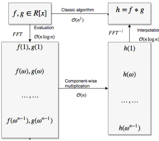
Figure 2.1:FFT-based univariate polynomial multiplication
The whole procedure needs 92nlogn+O(n) arithmetic operations inA(see [17] Theorem 8.18 for details) so that the multiplication time of FFT-based multiplication is
M(n)=O(nlogn) (2.25)
Table2.1 gives the multiplication time for some popular fast multiplication algorithms.
Table 2.1: Multiplication time of different algorithms.
Algorithm M(n)
Classic Algorithm O(n2) Karatsuba’s Algorithm O(n1.585) Toom-3 O(n1.465)
Toom-4 O(n1.404)
FFT-based Algorithm O(nlogn) Sch¨onhage-Strassen’s Algorithm O(nlognlog logn)
2.5
Big
O
and
Θ
notations
When analyzing the complexity of algorithms, we use the big Oand theΘ notations, where big Ogives a asymptotic upper bound of a function and Θgives an order of magnitude of a function.
Definition 4 We say that g(n)is in theorder of magnitudeof f(n)and write f(n)∈Θ(g(n))if there exists two strictly positive constants c1and c2 such that for n big enough we have
0≤c1g(n)≤ f(n)≤ c2g(n)
Definition 5 We say that g(n)is anasymptotic upper boundof f(n)and write f(n) ∈ O(g(n)) if there exists a strictly positive constant c2 such that for n big enough we have
0≤ f(n)≤ c2g(n)
The bigO(andΘ) can also be used with multiple variables as follows. Let f,gbe functions, with positive real values, and depending on a vector~n= (n1, . . . ,nq) of non-negative integers.
We write f(~n)∈ O(g(~n)) whenever there exits two strictly positive constantMandC, such that for all~nsatisfyingni ≥ Mfor all 1≤i≤qwe have 0≤ f(~n)≤Cg(~n) [7].
For us the multivariate version of bigOgiven above is too strong. We define the multivariate bigOas follows for two integer variablesw,n.
Definition 6 f(w,n) ∈ O(g(w,n)) means that there exist three positive integer constants w1, w2, n1, with w1 < w2, and a positive real constant c such that for all positive integers w,n, if w1 ≤w≤w2 and n≥n1both hold, then we have f(w,n)≤ cg(w,n).
2.6
Syntax of pseudo-code
We use the following syntax in all the pseudo-code of the algorithms:
• a:=bassigns valuebto variablea
• a=breturns true ifais equal tob, otherwise returns false
• ~xis a vector
• xiis thei-th element in~x
Here are some notations for the C code we present in the paper:
• usfixn64is the type of unsigned 64-bit integer
• sfixnis the type of signed 64-bit integer
• U64 MASKis defined as 264−1
Chapter 3
Generalized Fermat prime field arithmetic
Small prime field arithmetic has been implemented in different computer algebra systems. With the help of tricks like Montgomery’s reduction, this can be done efficiently, but the small char-acteristic restricts the precision to a single machine word. Multi-precision numbers can be handled using the Chinese Remainder Theorem. Nevertheless, for certain algorithms in com-puter algebra, like modular methods for polynomial systems [1, 8, 2] it is desirable to use prime fields of large characteristic, thus computing modulo prime numbers with size on the order of several machine words.
Since modular methods for polynomial systems rely on polynomial arithmetic, those large prime numbers must support FFT-based algorithms, such as FFT-based polynomial multiplica-tion. This leads us to consider the so-called Generalized Fermat prime numbers.
Then-th Fermat number can be denoted byFn = 22 n
+1. This sequence of numbers plays an essential role in number theory. Arithmetic operations on fields based on Fermat numbers are simpler than those of other arbitrary prime numbers since 2 is the 2n+1-th primitive root of unity moduloFn. But, unfortunately, the largest Fermat prime number known now is F4. This
triggered the interests of finding Fermat-like numbers. Generalized Fermat numbersare one of these kinds.
Numbers that are in the form ofa2n +b2n witha,bany co-prime integers, wherea> b>0 andn>0 hold, are calledgeneralized Fermat numbers. Among all, those withb= 1 are of the most interest; we commonly write generalized Fermat numbers of the forma2n+1 asFn(a). For
a generalized Fermat number p, we useZ/pZto represent the finite fieldGF(p). In particular, in the fieldZ/Fn(a)Z,ais a 2n+1-th primitive root of unity. But with the binary representation
of numbers on computers, the arithmetic operations on such fields are not as simple as those of Fermat numbers. To solve this problem, a special kind of generalized Fermat number is defined in the previous work of our research group [4].
Any integer in the form ofFn(r)= (2w±2u)k+1 is called a sparse radix generalized Fermat
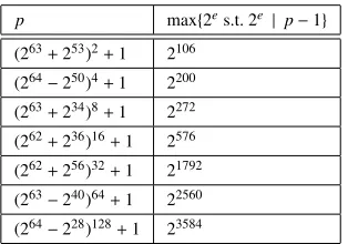
number, wherew > u ≥ 0. Table 3.1 lists some sparse radix generalized Fermat numbers that are primes. For each prime p=Fn(r),kis some power of 2 and the prime writes as p= rk+1.
In the same table, the number 2e is the largest power of 2 that divides
p−1, which gives the maximum length of a vector to which we can apply a 2-way FFT algorithm.
In Section 3.1, we will introduce how we can use the radix-rrepresentation to represent the elements inZ/pZ. Section 3.2 will introduce the special primitive roots of unity that can benefit us when computing FFT overZ/pZ, and will give an algorithm on how to get those primitive
Table 3.1: SRGFNs of practical interest. p max{2es.t.2e | p−1} (263+253)2+1 2106
(264−250)4+1 2200
(263+234)8+1 2272
(262+236)16+1 2576 (262+256)32+1 21792
(263−240)64+1 22560
(264−228)128+1 23584
roots. Next, in Section 3.3, we will show the algorithm for doing addition and subtraction in Z/pZ. In Section 3.4, we will discuss how we can multiply any elements with a power of r efficiently. This idea fits in F¨urer’s algorithm that, for DFT on certain points, multiplication by the particular primitive roots can be done in a very cheap way. Last, in Section 3.5, we give the basic algorithm on multiplication between two arbitrary elements inZ/pZ.
3.1
Representation of
Z
/
p
Z
In the finite prime field Z/pZ, where p = rk +1, each element x is represented by a vector ~x=(xk−1, . . . ,x0) of lengthk. We restrict all the coefficients to be non-negative integers so that we have
X ≡ xk−1rk−1+xk−2rk−2+· · ·+x1r+ x0 mod p (3.1) The following two cases make the representation unique for each element:
1. Whenx≡ p−1 mod pholds, we have xk−1= randxk−2 =· · ·= x0= 0. 2. When 0≤ x< p−1 holds, we have 0≤ xi < rfori=0, . . . ,k−1.
We can also use a univariate polynomial fx ∈ Z[R] to represent x: we write fx = P k−1
i=0 xiRi,
such that x≡ fx(r) mod p.
When computing the representation~xof a numberx< p, the case wherex= p−1 is trivial, since we can directly set xk−1 torand xk−2, . . . ,x0to 0. Consider the case 0 ≤ x < p−1. Let qk = 0 and sk = x. Then, for 0 ≤ i < k, qi and si are the quotient and the remainder in the
Euclidean division ofsi+1byri so that we have xi =qi, for 0≤ i<k.
3.2
Computing the primitive root of unity in
Z
/
p
Z
Recall that for anynthat divides p−1, we can use algorithm 2.1 to find ann-th primitive root of unity inZ/pZ. Now we want to consider the case of finding anN-th primitive root of unity ωinZ/pZsuch thatωN/2k = r holds. Indeed, computing a DFT at suchω on a vector of size N would take advantage of the fact that multiplying by a power ofrcan be done in linear time, see Section 3.4.
3.3. Addition and subtraction inZ/pZ 17
Algorithm 3.1PrimitiveN-th rootω∈Z/pZsuch thatωN/2k =r
1: procedureBigPrimeFieldPrimitiveRootOfUnity(N,r,k,g) 2: a:= gN/2k
3: b:= a 4: j:=1
5: whileb, rdo 6: b:= a b 7: j:= j+1 8: end while
9: ω :=gj
10: return(ω)
11: end procedure
From the definition of generalized Fermat prime numbers we know thatris a 2k-th primi-tive root of unity inZ/pZ, where p=rk+1. WhilegN/2k is a 2k-th root of unity, it must equal to some power ofr, sayrt mod pfor some 0 ≤t < 2k. Let jbe a non-negative integer,qand
sare the quotient and the remainder of jin the Euclidean division by 2k, so we have
j=q·2k+s (3.2)
and
gjN/2k = g2kq+sgN/2k =gsgN/2k = (gN/2k)s =rts (3.3) By the definition of primitive root of unity, the powersrtsare pairwise different for 0≤ s<
2kand for some si,rtsi = rholds. Hence, for some ji = qi·2k+ si, we will have (gN/2k)ji = r.
Thenω =gji is the primitive root of unity that we want.
3.3
Addition and subtraction in
Z
/
p
Z
Algorithm 3.2Computingx+y∈Z/pZforx,y∈Z/pZ 1: procedureBigPrimeFieldAddition(~x,~y,r,k)
2: computezi = xi+yi inZ/pZ, fori=0, . . . ,k−1,
3: letzk =0,
4: for i = 0, . . . ,k− 1, compute the quotient qi and the remainder si in the Euclidean
division ofzibyr, then replace (zi+1,zi) by (zi+1+qi,si),
5: ifzk =0 then return (zk−1, . . . ,z0),
6: ifzk =1 andzk−1 =· · · =z0 =0, then letzk−1 =rand return (zk−1, . . . ,z0),
7: let i0 be the smallest index, 0 ≤ i0 ≤ k, such thatzi0 , 0, then let zi0 = zi0 −1, let
z0 = · · ·=zi0−1 = r−1 and return (zk−1, . . . ,z0).
8: end procedure
In this theoretical algorithm, we use a Euclidean division to compute the carry and the remainder of xi +yi, which requires a division and a subtraction operation. But in practical
implementation, we can avoid the expensive division. The following lists the C code we used in the BPAS library.
According to the method in 3.1, each component of~xand~yis in the range of [0,k−1] for 0≤i≤ k−2 andxk−1,yk−1 ∈[0,k], so that we can safely say that the results of the component-wise addition will not be greater than 2r−2 for the first k−1 pairs of component. Hence, if the sum is greater thanr, we can simply subtract the result byrand set the carry to 1, instead of using an Euclidean division. For the last pair xk−1andyk−1, the two special cases are one of them is equal torand both of them are equal tor. For the first case, the maximum sum ofxk−1 andyk−1 is 2r−1, there is no difference from the previous method.
Now, let’s consider the second case where both xk−1 and yk−1 are equal to r. And all of the other components in the vectors are 0, such that both x andy are equal to rk. When we add the two components together uk−1 is equal to 2r and by using line 9 to 11 from listing 3.1, we have uk−1 = r and carry = 1. Then uk−1 is the first ui that is not 0. In line 33, we
have uk−1 = uk−1 − 1 = r − 1 and in line 31 we set ui = r − 1 for 0 ≤ i < k − 1. The
result we get is ui = r − 1 for 0 ≤ i < k, that is equal to u ≡ −2 mod p, indeed that
x+y ≡ rk+rk ≡ 2(p−1) ≡ 2p−2 ≡ −2 mod p. So far we have proved that our algorithm
works correctly and efficiently for all of the cases.
1 sfixn* addition (sfixn * x, sfixn *y, int k, sfixn r) {
2 short c = 0;
3 short post = 0;
4 sfixn sum = 0;
5 int i = 0;
6
7 for (i=0;i < k;i++) {
8 sum = x[i] + y[i] + c;
9 if (sum >= r ) {
10 c = 1;
11 x[i] = sum - r;
12 }
13 else {
14 x[i] = sum;
15 c = 0;
3.4. Multiplication by power ofrinZ/pZ 19
17 }
18
19 if (c > 0) {
20 post = -1;
21
22 for (i = 0; i < k; i++) {
23 if (x[i] != 0) {
24 post = i;
25 break;
26 }
27 }
28
29 if (post >= 0) {
30 for (i = 0; i < post; i++) {
31 x[i] = r - 1;
32 }
33 x[post] - -;
34 }
35 else {
36 x[k-1] = r;
37 for (i = 0;i < k-1; i++) {
38 x[i] = 0;
39 }
40 }
41 }
42
43 return x;
44 }
Listing 3.1: Addition in a Generalized Fermat Prime Field
Similarly, we have an algorithm BigPrimeFieldSubtraction(~x,~y,r,k) for computing ←x−−−→y represents (x−y)∈Z/pZ.
3.4
Multiplication by power of
r
in
Z
/
p
Z
case that 0<i<k, we have the following equation:
xri ≡ (xk−1rk−1+i+· · ·+x0ri) mod p
≡
j=k−1 P
j=0
xjrj+i mod p
≡
h=k−1+i
P
h=i
xh−irh mod p
≡ (
h=k−1 P
h=i
xh−irh− h=k−1+i
P
h=k
xh−irh−k) mod p
We see that for all 0≤ i≤ 2k, x·riis reduced to some shift and a subtraction. We call this
process cyclic shift. The following gives the C implementation in the BPAS library.
1 sfixn* MulPowR(sfixn *x,int s, int k, sfixn r){
2 sfixn *a =(sfixn*)calloc(sizeof(sfixn) ,k);
3 sfixn *b =(sfixn*)calloc(sizeof(sfixn) ,k);
4 sfixn *c =(sfixn*)calloc(sizeof(sfixn) ,k);
5 s = s%(2 * k);
6 if (s == 0)
7 return x;
8 else if (s == k)
9 return BigPrimeFieldSubtraction(c,x,k,r);
10 else if ((s > k) && (s < (2 * k))){
11 s = s - k;
12 x = BigPrimeFieldSubtraction(c,x,k,r);
13 }
14 int i;
15 for (i = 0; i < (k - s); i++)
16 b[i + s] = x[i];
17 for (i = k - s; i < k; i++)
18 a[i - (k - s)] = x[i];
19 if(x[k-1] == r){
20 a[s-1] -=r;
21 a[s] ++;
22 }
23 return BigPrimeFieldSubtraction(b,a,k,r);
24 }
Listing 3.2: Multiplication by power if r in a Generalized Fermat Prime Field
3.5
Multiplication between arbitrary elements in
Z
/
p
Z
According to Section 3.1, we use the univariate polynomials fx, fy ∈ Z[R] to represent input elements x,y ∈ Z/pZrespectively. Algorithm 3.3 computes the product x·y ∈ Z/pZ. In the first step, we multiply the two polynomials overZand compute the remainder fuof the product
modulo Rk +1. Then, we convert all the coefficients of fu into the radix-r representation in
3.5. Multiplication between arbitrary elements inZ/pZ 21
Algorithm 3.3Computingx·y∈Z/pZforx,y∈Z/pZ 1: input:
- an integerkand radixr,
- two polynomials fxand fy whose coefficient vectors are~x,~y.
2: output:
- a vector~u
3: procedureBigPrimeFieldMultiplication(fx, fy,r,k)
4: fu(R) := fx(R)· fy(R) .computing fxtimes fy inZ[R]
5: fu(R) := fu(R) mod (Rk+1) .we get fu(R)=Pki=−10ui ·Ri
6: ~uis the coefficient vector of fu
7: for0≤ i<kdo
8: u~i := ui ∈Z/pZ .compute a radix representation of eachui using method in 3.1
9: end for
10: ~u:= u~0 .add all theuitogether using the algorithm 3.2
11: for1≤ i<kdo
12: ~u:=BigPrimeFieldAddition(~u, ~ui,k,r)
13: end for
14: return~u
15: end procedure
Optimizing multiplication in Generalized
Fermat prime fields
In this chapter, we will discuss how to multiply two arbitrary elements in Z/pZ efficiently using FFT, when p is a Generalized Fermat prime. Firstly, in Section 4.1, we outline two algorithms that we can use for this multiplication: one is based on polynomial multiplication (see Section 4.1.1) and the other one is based on integer multiplication by means of the GMP library [18] (see Section 4.1.2). Then, in Section 4.2 we provide detailed complexity analysis on the two approaches. Finally, in Section 4.3, we present the implementation of the FFT-based polynomial-based multiplication. We break down the algorithm into sub-routines and explain in details for each part. The C functions that we use can be found in Appendix A.
4.1
Algorithms
Let pbe a Generalized Fermat prime. When actually implementing the multiplication of two arbitrary elements in the fieldZ/pZ, we use two different approaches. In the first approach, we follow the basic idea explained in Chapter 3 (see Algorithm 3.3) which treats any two elements x,yin the field as polynomials fx, fyand uses polynomial multiplication algorithms to compute
the product xy. The other approach involves converting the elements x,y from their radix-r representation into GMP integer numbers and letting the GMP library [18] do the job.
4.1.1
Based on polynomial multiplication
In Section 3.5 we gave the basic algorithm for multiplying two arbitrary elements of Z/pZ based on polynomial multiplication. In practice, there are more details to be considered in order to reach high-performance. For instance, how do we efficiently convert a positive integer in the range (o,r3) into radix-rrepresentation.
Let us consider how to calculateu = x y mod pwith x,y,u∈Z/pZ. Here we want to use the polynomial representation of the elements in the field, that is, fx(R)= xk−1Rk−1+· · ·+x1R+ x0 and fy(R) = yk−1Rk−1+· · ·+y1R+y0. The first step is to multiply the two polynomials fx
and fy. We can use different polynomial multiplication algorithms depending on the value of
4.1. Algorithms 23
k. Let us look at the expansion of fu. Recall that taking a polynomial modulo byRn+1 means
replacing every occurrence ofRn by−1.
fu(R) = fx(R)· fy(R) mod (R k+
1)
=
2k−2 X
m=0
i+j=m
X
0≤i,j<k
xiyjRm mod (Rk+1)
= (xk−1y0+xk−2y1+xk−3y2+· · ·+ x1yk−2+x0yk−1)Rk−1
+ (xk−2y0+xk−3y1+· · ·+x1yk−3+ x0yk−2−xk−1yk−2)Rk−2
+ (xk−3y0+xk−4y1+· · ·+x0yk−3− xk−1yk−2− xk−2yk−1)Rk−2
. . .
+ (x1y0+x0y1−xk−1y2− · · · −x2yk−1)R
+ (x0y0−xk−1y1− · · · −x1yk−1)
=
k−1 X
m=0 (
i+j=m
X
0≤i,j<k
xiyj− i+j=k+m
X
0≤i,j<k
xiyj)Rm
Each coefficientui of fuis the combination ofkmonomials, so the absolute value of each
ui is bounded over by k· r2 which implies that it needs at most blogk +2 logrc+ 1 bits to
be encoded. Sincek is usually between 4 to 256, a radixrrepresentation of ui of length 3 is
sufficient to encodeui. Hence, we denote by [ci,hi,li] the 3 integers uniquely given by:
1. ui =cir2+hir+li,
2. 0≤hi,li <r.
3. ci ∈[−(k−1),k],
4. ciui ≥0 holds.
Then, we can rewrite:
fu(R) = fx(R)· fy(R) mod (Rk+1)
= (c0R2+h0R+l0)+(c1R2+h1R+l1)R+(c2R2+h2R+l2)R2+· · ·
+(ck−2R2+hk−2R+lk−2)Rk−2+(ck−1R2+hk−1R+lk−1)Rk−1
=
k−1 X
i=0
(ciR2+i+hiR1+i+liRi)
Now we obtain three vectors~c=[c0,c1, . . . ,ck−1],~h= [h0,h1, . . . ,hk−1] and~l= [l0,l1, . . . ,lk−1] with k coefficients each. As we shift~c to the right twice and~hto the right once, we deduce three numbersc,h,lin the radix-rrepresentation.
c = ck−3rk−1+ck−4rk−2+· · ·+c0r2+ck−2r+ck−1 h = hk−2rk−1+hk−3rk−2+· · ·+h1r2+h0r+hk−1
At last we need two additions inZ/pZ to compute the resultu = c+h+l = x y mod p withx,y,u∈Z/pZ.
Now we consider the question of how to calculate [l,h,c] quickly. Because of the special structure of r, where only two bits are 1, we can use some shift operations to reduce the bit complexity and save on the cost of divisions. Differentr’s have different non-zero bits, but for clarity of presentation we use a particular radixr, namelyr =263+234, for the primeP= rk+1
withk =8.
Let xi,yjbe any two digits in the radixrrepresentation ofx,y∈Z/pZ. Since 0 ≤ xi,yj ≤ r
holds, we have
xiyj = (xi0+xi1r) (yj0+yj1r)
= xi0yj0+(xi0yj1+xi1yj0)r+xi1yj1r2
where 0 ≤ xi0,yj0 < r, andxi1,yj1 ∈ {0,1}. Hence, we have 0 ≤ xi0yj1, xi1yj0, xi1yj1 < r. We only need to consider the case ofxi0yj0, where 0≤ xi0yj0 <r2 <2127. We can rewrite
xi0yj0 = (a0+a1232)(b0+b1232)
= a0b0+a0b1232+a1b0232+a1b1264
= c0+c1264.
Notice that a0,a1,b0,b1 are in [0,232), using addition and shift operation, we can rewrite xi0yj0into the formc0+c1264, wherec0 <264andc1< 263. Then, we have:
xi0yj0 = c0+c1264
= c0+c012
63 where c0
1= 2c1,0≤c01 <2 64
= c0+c01(263+234)−c01234
= c0+c01r−c01234,
where the partc0+c01rcan be rewritten into the form ofl+hr+cr
2easily.
Forc0 12
34, where 0≤c0 1 <2
64 holds, we observe:
c01234 = (d0+d1229)234 with 0≤d0 <229,0≤ d1< 235
= d0234+d1263
= d0234+d1(263+234)−d1234
= (d0−d1)234+d1r
= (e0+e1229)234+d1r with |e0|< 229,|e1|< 26
= (e0−e1)234+e1r+d1r.
Since|(e0−e1)234|< rholds, the numberc01234can easily be rewritten into the form ofl+hr+cr2. We add the (l,h,c)-representations of each part together, with some normalization we can get the result we need where xiyj = l+h r+c r2.
4.1. Algorithms 25
Algorithm 4.1An algorithm for rewritingxiyjintol+hr+cr2
1: procedureRewrite([l,h,c]=[xi,yj])
2: if xi ≥ rthen
3: xi1 := 1 4: xi0 := xi−r
5: else
6: xi1 := 0 7: xi0 := xi
8: end if . xi = xi0+ xi1r
9: ifyi ≥ rthen
10: yi1:= 1 11: yi0:= yi−r
12: else
13: yi1:= 0 14: yi0:= yi
15: end if .yi =yi0+yi1r
16:
17: [v1,v2,v3] := [0,xi0yi1,0]; . xi0yi1r
18: [v4,v5,v6] := [0,xi1yi0,0]; . xi1yi0r 19: [v7,v8,v9] := [0,0,xi1yi1]; . xi1yi1r2 20:
21: c0 := xi0yi1−264 22: c1 :=(xi0yi1)>>64
23: c01 :=2c1 .xi0yi0= c0+c1264= c0+c01263 24: ifc0 ≥rthen
25: [v10,v11,v12] := [c0−r,1,0] 26: else
27: [v10,v11,v12] := [c0,0,0]
28: end if .c0= v10+v11r+v12r2 29: ifc01 ≥rthen
30: [v13,v14,v15] := [0,c01−r,1] 31: else
32: [v13,v14,v15] := [0,c01,0]
33: end if .c0
1r= v13+v14r+v15r 2;
34:
35: d1 :=c01 >>29; 36: d0 :=c01−d1 <<29; 37: e1 :=(d0−d1)>>29; 38: e0 :=(d0−d1−e1 <<29);
39: [v16,v17,v18] := [(e0−e1)<<34,e1+d1,0]; 40:
41: [l,h,c] := [v1+v4+· · ·+v16,v2+v5+· · ·+v17,v3+v6+· · ·+v18]; 42: return[l,h,c];
The following algorithm is to calculateu= x y mod p.
Algorithm 4.2Computingu=x y∈Z/pZforx,y∈Z/pZusing polynomial multiplication
1: procedurePolynomialMultiplication(~x,~y,r,k) 2: Multiply fu(R)= fx(R)· fy(R) mod (Rk +1)
3: form from 0 to k - 1do
4: [li,hi,ci]= P i+j=m
0≤i,j<kxiyj−
Pi+j=k+m 0≤i,j<k xiyj
5: end for
6: .The above k clauses can be executed in parallel
7:
8: S hi f tT oRight[c0,c1, . . . ,ck−1]
9: S hi f tT oRight[ck−1,c0, . . . ,ck−2] 10: S hi f tT oRight[h0,h1, . . . ,hk−1] 11: u= c+h+l mod p
12: returnu 13: end procedure
4.1.2
Based on integer multiplication
This approach is more straight forward. For two numbersxandyin our radixrrepresentation, we map the vectors ~x and ~y to two polynomials fx, fy ∈ Z[R]. Then we evaluate the two polynomials atr, which gives us two integersXandY, using integer multiplication and modulo operation gives the resultU = X Y mod p. At last, we only need to convert the product back to the radixrrepresentation. See Algorithm 4.3.
Algorithm 4.3Computingx y∈Z/pZforx,y∈Z/pZusing integer multiplication
1: procedureIntegerMultiplication(~x,~y,r,k,p)
2: X :=0Y := 0 .X andY are GMP integers
3: forifromk−1 to 0do
4: X:= X·r+xi
5: Y :=Y·r+yi
6: end for
7: U :=(X·Y) mod p
8: returnGeneralizedFermatPrimeField(U) 9: end procedure
4.2
Analysis
4.2. Analysis 27
In the following analysis, we compute u = x · y, where x = xk−1rk−1 + · · · + x0 and y = yk−1rk−1 +· · · + y0 are two numbers in our Generalized Fermat Prime Field, with radix
rrepresentation. Let Mbe a multiplication time and letω be the number of bits in a machine word. We want to analyze the complexity of multiplication with different approaches.
4.2.1
Based on polynomial multiplication
We viewxandyas polynomials fx and fyin a variableRwith integer coefficientsx0, . . . ,xk−1 and y0, . . .yk−1, whose bit sizes are at most that of one machine word. First step in our mul-tiplication is to multiply fx and fy inZ[R], obtaining fu = u2k−2R2k−2 + · · ·+u0. The
multi-plication time of multiplying two polynomials of degree less thank isM(k). The complexity of multiplying each pair of coefficients is M(ω) and the largest bit size of the coefficients of fuisω+k, so the maximum complexity of each operation in the polynomial multiplication is
max(M(ω),Θ(ω+k)), which gives us the total complexity of this step:
M(k) max(M(ω),Θ(ω+k)) (4.1)
In the next step, we compute the remainder of fu w.r.t Rk + 1. We should notice that
computing the remainder here is the same as computing fu mod (Rk +1) that is using−1 to
replace everyRk. So, for each term in fu, if the degree is greater thank−1, reduce the degree
bykand reverse the sign for the coefficient. Combining the terms with the same degree gives the final result of this step, fu = fxfy mod (Rk+1)=uk−1Rk−1+· · ·+u0. The total number of operations that we need to compute the remainder is in the order ofΘ(k), the bit complexity of each operation isΘ(ω+k), thus the complexity of this step is:
Θ(kω) (4.2)
Next, we want to write each ui asli +hir+cir2 with 0 ≤ li,hi,ci < rusing two divisions
(one byr2and one byr), we get three vectors [l0, . . .lk−1], [h0, . . .hk−1] and [c0, . . .ck−1]. Using cyclic shift on the three vectors, we obtain three numbers in radix r format: zl,zh,zc. We need
2kdivisions in machine word size and three cyclic shifts for this step in total. So the complexity is:
Θ(kM(ω)) (4.3)
The last step in this approach is to add three numbers,zl,zh,zc, together using two additions
inZ/pZ. The complexity is:
Θ(kω) (4.4)
We can see that the second step has the greatest complexity 4.2. Thus, the total complexity of the approach based on polynomial multiplication is in the order of:
4.2.2
Based on reduction to integer multiplication
In this approach, we convert two numbers in our radix r representation x andy into two big integersXandY. Then we multiply them together as integers and convert the product to radix-rrepresentation. All of the operations we use in this method can be performed with the GMP library [18].
The GMP library chops the numbers into several parts which are called “limbs”. For numbers with different numbers of limbs, GMP uses different multiplication algorithms. Let us consider the case of multiplication between two equal size numbers with N limbs each. For the base case with no threshold, the naive long multiplication is used with complexity of
O(N2). With the minimum of 10 limbs, GMP uses Karatsuba’s algorithm with complexity of
O(Nlog 3/log 2). Furthermore, multi-way Toom multiplication algorithms are introduced. Toom-3 is asymptoticallyO(Nlog 5/log 3), representing 5 recursive multiplies of 1/3 original size each while Toom-4 has the complexity ofO(Nlog 7/log 4). Though there seems an improvement over Karatsuba, Toom does more evaluation and interpolation so it will only show its advantage above a certain size. For higher degree Toom ‘n’ half is used. Current GMP uses both Toom-6 ‘n’ half and Toom-8 ‘n’ half. At large to very large sizes, GMP uses a Fermat style FFT multi-plication, following Sch¨onhage and Strassen. Herekis a parameter that controls the split, with FFT-k splitting the number into 2k pieces, leading the complexity toO(Nk/(k−2)). It meansk =7 is the first FFT that is faster than Toom-3. Practically, the threshold for FFT in the GMP library
is found in the range ofk = 8, somewhere between 3000 and 10000 limbs(See more in GMP
library [18] manual).
Firstly, we reduce xandytoXandY using the following method.
X =(((xk−1∗r)+xk−2)∗r· · ·+x1)∗r+x0 (4.6) which needsk−1 additions andk−1 multiplications with at most kωbits. Here, we still useMto represent the multiplication time. So, the complexity of this step is:
Θ(kM(kω)) (4.7)
Then we multiply X and Y using operation from the GMP library. Let U = X ·Y. The
complexity is
M(kω) (4.8)
At last,Uwritesu=uk−1rk−1+· · ·+u0usingk−1 divisions (byrk−1, . . . ,r). The complexity is:
Θ(kM(kω)) (4.9)
The total complexity of this approach is
4.3. Implementation withCcode 29
4.3
Implementation with C code
In this section we give some details of how we actually implement the multiplication between two arbitrary elements inZ/pZ. We follow the basic idea of algorithm 4.2 but there are more problems we need to solve.
Let fx(R), fy(R) represent x,y ∈ Z/pZ respectively. In the first step of the multiplication,
we need to compute fu(R) = fx(R) · fy(R) mod (Rk + 1) in Z/pZ, which is a Negacyclic
convolution. In Section 2.4, we introduced a fast algorithm to compute convolution, which is computing f(x)·g(x) mod (xn −1) for two polynomials f andgwith degree less than n. A
similar approach can be used for computing the negacyclic convolution.
Letq be a prime,ωbe an n-th primitive root of unity inZ/qZ, andθ be a 2n-th primitive root of unity inZ/qZ. Also we have two polynomials f(x) andg(x) with degree less thann, we use~a and~bto represent the coefficient vector of the f and g. First, we need to compute two vectors
~
A= (1, θ, . . . , θn−1) (4.11)
and
~
A0 =(1, θ−1, . . . , θ1−n
) (4.12)
The negacyclic convolution of f andgcan be compute as follow
~
A0·InverseDFT(DFT(A~·~a)·DFT(A~·~b)) (4.13)
All the dot multiplication between vectors are point-wise multiplication. The InverseDFT and DFTs are alln-point. We use unrolled inline DFTs in the implementation. The details of the DFTs are given in Chapter 5. This equation gives the following algorithm.
Algorithm 4.4 is to compute fx(R)·fy(R) mod (Rk+1) over a finite fieldZ/qZwithqbeing a machine word size prime and fx(R), fy(R) being two polynomials of degreek−1. ~xand~yare
Algorithm 4.4Computing fx(R)· fy(R) mod (Rk+1) inZ/qZusing Negacyclic Convolution 1: input:
- a prime numberqandkis a power of 2 withk|(q−1),
- two vectors~xand~yof k elements,contain the coefficients of polynomials fx(R) and
fy(R).
2: output:
- a vector~uthat contains the coefficients of polynomial fu(R)= fx(R)·fy(R) mod (Rk+
1)
3: procedureNegacyclicConvolution(~x, ~y, q, k)
4: ω:=PrimitiveRootOfUnity(q, k); . ωis the kth primitive root of unity ofq
5: θ:=PrimitiveRootOfUnity(q, 2 k); . θis the 2kth primitive root of unity ofq
6: for0≤ i≤k−1do
7: Ai :=θi mod q;
8: xi := xi·Ai mod q;
9: yi := yi·Ai modq;
10: end for
11:
12: ~x:= DFT(~x, ω,q,k); 13: ~y:= DFT(~y, ω,q,k); 14:
15: for0≤ i≤k−1do
16: ui := xi·yi mod q;
17: end for
18: ~u:= DFT(~u, ω−1 mod q,q,k) 19: for0≤ i≤k−1do
20: A0i :=θ−i mod q;
21: ui := 1k(ui·A0i) mod q;
22: end for
23: return~u 24: end procedure
Notice that for fxand fyin our Generalized Fermat Prime FieldZ/pZ, each coefficient is at most 63 bits. When computing fu(R)= fx(R)· fy(R) mod (Rk+1), the size of the coefficients
of fu can be at most logk+ (2· 63) = 126+ logk, which is more than one machine word,
so that we cannot do the computation using single-precision arithmetic. But, multi-precision arithmetic can be very expensive and would make the algorithm inefficient. So we use two machine word negacyclic convolution in stead of one using big numbers. Hence, we need to apply the Chinese Remainder Theorem (CRT) to get the result that we want.
Let p1andp2be two machine word size prime numbers, so that we haveGCD(p1,p2)= 1. Then we use the extended Euclidean division to getm1andm2that satisfy the following relation
4.3. Implementation withCcode 31
Letabe an integer and we have
a1 ≡a mod p1 (4.15)
a2 ≡a mod p2 (4.16)
Then we computea mod (p1p2) by
a ≡ a2p1m1+a1p2m2 mod (p1p2) (4.17)
= ((a2m1) mod p2)p1+((a1m2) mod p1)p2 (4.18)
Hence, for x,y ∈ Z/pZ, we compute u1 = x·y mod p1 andu2 = x·y mod p2, then use 4.18 to computeu = x·y mod (p1p2). With some normalization we will getu = x·y ∈ Z. LetR= k r2be the upper bound of (|u0|, . . . ,|uk−1|)∈Z. To get the correct answer, we need the following restrictions:
1. R≤ p1p2−1
2
2. the results we get from the CRT should be normalized so that they fall into the range of [−p1p2−1
2 ,
p1p2−1
2 ] If p1p2−1
2 < R, any result that is in the range of (
p1p2−1
2 ,R) and (−R,−
p1p2−1
2 ) will be inaccu-rate since the modular operation will make it in the range of [−p1p2−1
2 ,
p1p2−1
2 ].
As we mentioned before, all the results are in the range of (−R,R) in Z, which means
−p1p22−1 < ui < p1p2−1
2 hold. Hence, after all the normalization we will have all the results inZ without losing any accuracy.
The small primes p1 and p2 are hard coded into the algorithm for now, where both p1 =
4179340454199820289 andp2 =2485986994308513793 are 61-bit numbers. So, when
choos-ing the Generalized Fermat prime, we should be very careful because of the two restrictions. For these two primes p1 and p2, the size of the chosen Generalized Fermat prime number p= rk+1 should be as follows:
log p1p2−1
2 >log(k r
2) (4.19)
121> logk+2 logr (4.20)
logr <59 when k= 8 (4.21)
logr <58 when k= 16 (4.22)
logr <58 when k= 32 (4.23)
logr <57 when k= 64 (4.24)
As we know, the modular operation in 4.18 is expensive, so in the implementation we use what is calledreciprocal divisionto reduce the cost of the modular operations.
Let’s say we want to computea mod n, instead of doing one single modular operation, we pre-compute the value ofninv=1/n. Then we compute the result by
a−n·a·ninv≡a mod n (4.25)
Here, we only keep the integer part of a· ninv, so that n· a· ninv gives the quotient of the Euclidean division ofabyn.