A N EIKONAL MODEL FOR MULTIPARTICLE
PR O D U C TIO N IN H A D R O N -H A D R O N
SCATTERING
UCL
A
THESIS SUBMITTED TO THE UNIVERSITY COLLEGE LONDONFOR THE DEGREE OF DO CTO R OF PHILOSOPHY
IN THE Fa c u l t y o f Sc i e n c e
By
Ivan Borozan
D epartm ent of Physics and A stronom y
All rights reserved
INFORMATION TO ALL USERS
The quality of this reproduction is dependent upon the quality of the copy submitted.
In the unlikely event that the author did not send a complete manuscript and there are missing pages, these will be noted. Also, if material had to be removed,
a note will indicate the deletion.
uest.
ProQuest 10014378
Published by ProQuest LLC(2016). Copyright of the Dissertation is held by the Author.
All rights reserved.
This work is protected against unauthorized copying under Title 17, United States Code. Microform Edition © ProQuest LLC.
ProQuest LLC
789 East Eisenhower Parkway P.O. Box 1346
C on ten ts
L ist o f F igures 3
A b stra ct 4
D ecla ra tio n 6
D e d ic a tio n 7
A ck n ow led gem en ts 8
T h e A u th o r 10
1 In tro d u ctio n 11
1.1 In tro d u c tio n ... 12
1 .2 Q C D ... 13
1.2 .1 QCD L a g ra n g ia n ... 14
1.2.2 R enorm alization... 15
1.2.3 Asymptotic freedom ... 18
1.2.5 Scaling violation and the Altarelli-Parisi e q u a tio n s... 2 2
1.2.6 Parton distribution functions ... 28
1.3 Regge Theory and Total cross s e c t i o n s ... 29
1.3.1 Two body s c a t te r i n g ... 29
1.3.2 The S-matrix, unitarity and the optical th e o r e m ... 31
1.3.3 Regge T h e o r y ... 34
1.3.4 Conclusion... 36
2 M o n te Carlo M eth o d s 37 2.1 In tro d u c tio n ... 38
2 .2 Random Number G en erato rs... 38
2.2 .1 Multiplicative Linear Congruential G e n e ra to rs ... 39
2.2 . 2 Compound Multiplicative Congruential G e n e r a t o r s ... 40
2.3 Distribution functions and Non-Uniform G e n e ra to rs ... 41
2.3.1 Transformation method ... 42
2.3.2 Rejection M e th o d ... 42
2.4 Integral e v alu a tio n s... 43
2.4.1 Monte Carlo vs q u a d ra tu re ... 44
2.5 Variance r e d u c t i o n ... 46
2.5.1 Stratified S a m p lin g ... 46
2.5.2 Importance S am p lin g ... 46
2.6 C onclusion... 48
Contents 4
3 E ven t gen erators 49
3.1 In tro d u c tio n ... 50
3.2 Hadron-Hadron in te r a c tio n s ... 50
3.2.1 The inclusive jet cross section in LO a p p ro x im a tio n ... 52
3.3 Final and Initial state parton sh o w ers... 55
3.3.1 Final State Parton S h o w e r... 55
3.3.2 Initial State Parton Shower ... 58
3.3.3 Hadronisation P r o c e s s ... 59
3.4 Event G e n e r a to rs ... 60
3.4.1 Event g e n e r a tio n ... 61
3.4.2 Event generation d e sc rip tio n ... 61
3.5 C onclusion... 63
4 J e t physics and th e u n d erlyin g even t 64 4.1 In tro d u c tio n ... 65
4.2 Kinematic v a ria b le s ... 65
4.3 Jets ... 67
4.3.1 CDF and D 0 Cone Algorithms and jet d e f i n it i o n ... 70
4.4 The Underlying event in Hard Scattering P r o c e s s e s ... 72
4.4.1 Charged particle jet definition... 74
4.4.2 Study of particle correlations in azimuthal a n g l e ... 75
4.4.3 Minimum-maximum region a n a ly s is ... 78
4.4.4 Transverse Cone a n a ly s is... 82
4.5 Summary ... 8 8 5 H ard M u ltip a rticle In tera ctio n M o d el 89 5.1 In tro d u c tio n ... 90
5.1.1 M ultiparton In te ra c tio n s ... 90
5.2 M ultiparton Interactions in the pp e n v iro n m e n t... 92
5.2.1 M ultiparton Interaction I m p le m e n ta tio n ... 95
5.2.2 Study of particle correlations in azimuthal angle... 97
5.2.3 Proton radius as a p a r a m e t e r ... 99
5.2.4 C onclusion... 104
6 Eikonal M o d el 111 6.1 In tro d u c tio n ...112
6 . 2 Introduction to the Eikonal M o d el... 112
6.3 Expression for the e i k o n a l ...114
6.3.1 The expression for Xtotai{b,s)...115
6.4 The Monte Carlo implementation of hard and soft p r o c e s s e s ...118
6.4.1 Assumptions behind the soft subprocess ...118
6.4.2 Implementation of the soft process ...120
6.5 Study of particle correlations in azimuthal a n g l e ...1 2 2 6.5.1 The invariance of the model to p t m i n ...125
6.5.2 U A l and LHC d a ta ... 136
Contents 6
6 . 6 C onclusion... 139
7 C on clu sion s and fu tu re w ork 144
7.1 C onclusion... 145
1.1 One loop Feynman diagram s... 17
1 . 2 Experimental tests of the QCD running coupling [5]... 20
1.3 Illustration of an DIS collision... 2 1 1.4 Scaling of the F2 structure function taken from [2] ... 23
1.5 Real part of the NLO contribution to j*q —> g... 24
1.6 Virtual part of the NLO contribution to 7*g —)■ g... 25
1.7 NLO contribution from gluon annihilation... 26
1.8 QCD fits to muon-proton DIS F2 taken from [2] ... 27
1.9 Parton density distributions as functions of x for = 20 GeV^ taken from [11]... 29
1.10 The scattering process in the s channel of eq.1.55... 30
1 .1 1 The optical theorem... 34
1 . 1 2 The p (o), u (□), (j) (A) and tt (•) trajectories. The p trajectory has been continued as measured in 7r~p —)■ rjn taken from [13]... 35
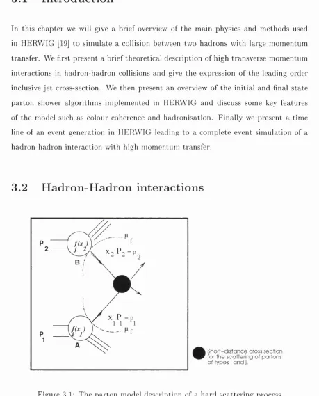
3.1 The parton model description of a hard scattering process ... 50
List of Figures
4.2 Illustrations of a) a hard subrocess occurring in a pp collision with
rem nant-rem nant interactions and b) non-diffractive soft interaction in
a pp collision... 6 8
4.3 Event with six charged particles pt>0.5 GeV and t; < 1 and five jets
(radius in rj — (f> space R = 0.7)... 74
4.4 Toward, away and transverse regions from the leading in pt jet (see [35]).
The angle A(f) = (j> — is the relative azimuthal angle between charged
particles and the direction of j e t # l ... 76
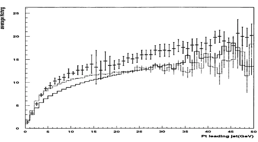
4.5 The average total number of charged particles in the event as a function of
Pt (leading charged jet). HERWIG + Underlying Event model (solid line)
simulated data, experimental CDF data [35] (data points)... 78
4.6 The average number of charged particles as a function of Ft (leading charged
jet) in the toward region. HERWIG 4- Underlying Event model (solid line)
simulated data, experimental CDF data [35] (data points). Charged particles
arising from the break-up of the beam and target (dotted line) and charged
particles that result from the outgoing jets initial and final-state radiation
(dotted dashed line) are shown separately... 79
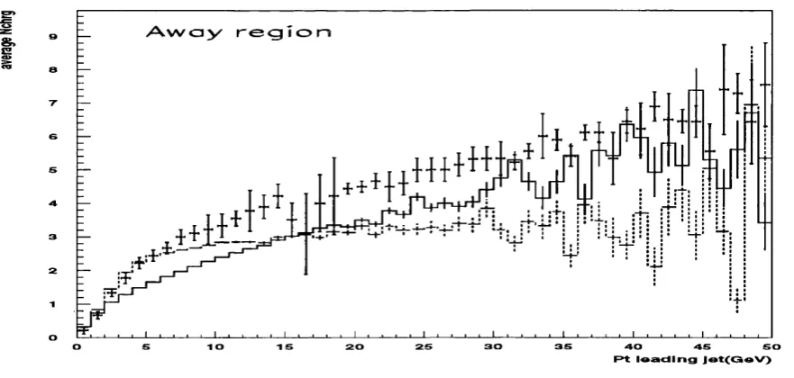
4.7 The average number of charged particles as a function of Ft (leading charged
jet) in the away region. HERWIG -f Underlying Event model solid line
simulated data, experimental CDF data [35] (data points). Charged particles
arising from the break-up of the beam and target (dotted line) and charged
particles that result from the outgoing jets initial and final-state radiation
(dotted dashed line) are shown separately... 79
4.8 The average number of charged particles as a function of Pt (leading charged
jet) in the transverse region. HERWIG + Underlying Event model solid line
simulated data, experimental CDF data [35] (data points). Charged particles
arising from the break-up of the beam and target (dotted line) and charged
particles that result from the outgoing jets initial and final-state radiation
(dotted dashed line) are shown separately. ... 80
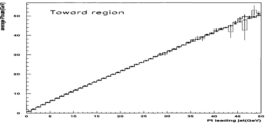
4.9 The average Pt sum of charged particles as a function of Pt (leading charged
jet) in the toward region. HERWIG + Underlying Event solid line simulated
data, experimental CDF data [35] (data points). Charged particles arising
from the break-up of the beam and target (dotted line) and charged particles
that result from the outgoing jets initial and final-state radiation (dotted
dashed line) are shown separately... 80
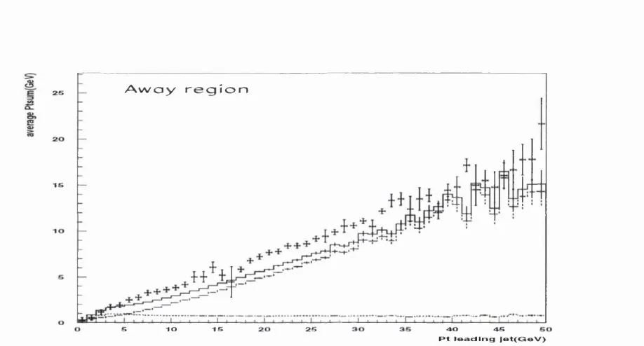
4.10 The average Pt sum of charged particles as a function of Pt (leading charged
jet) in the away region. HERWIG -f Underlying Event model solid line
simulated data, experimental CDF data [35] (data points). Charged particles
arising from the break-up of the beam and target (dotted line) and charged
particles that result from the outgoing jets initial and final-state radiation
(dotted dashed line) are shown separately... 81
4.11 The average Pt sum of charged particles as a function of Pt (leading charged
jet) in the transverse region. HERWIG 4- Underlying Event model (solid
line) simulated data, experimental CDF data [35] (data points). Charged
particles arising from the break-up of the beam and target (dotted line) and
charged particles that result from the outgoing jets intial and final state
radiation (dotted dashed line)... 81
4.12 The transverse region (left) split in two, the transverse maximum (Max)
and minimum (Min) parts (right)... 82
List of Figures 10
4.13 The average scalar pt sum of the trans-Max and trans-Min charged particles
as a function of Pt (leading charged jet) in the transverse region. Solid (Max)
and hollow (Min) circles are the experimental CDF data [35], the solid line
the corrected theoretical data from HERWIG 4- Underlying Event model. . . 83
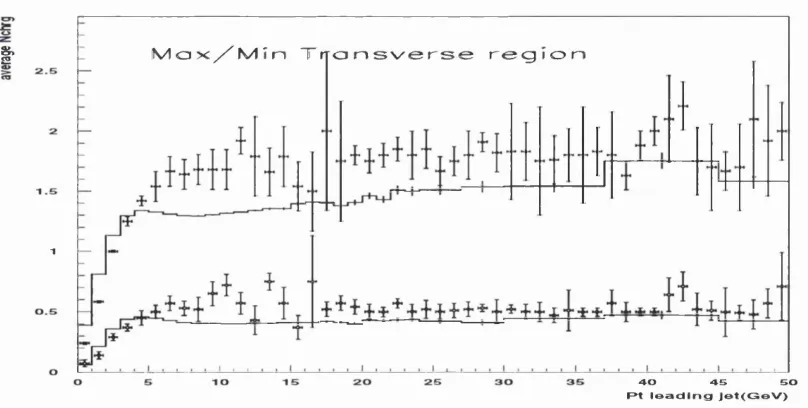
4.14 The average number of trans-Max and trans-Min charged particles as a func
tion of Ft (leading charged jet) in the transverse region. Solid (Max) and
hollow (Min) circles are the experimental CDF data [35], the solid line the
corrected theoretical data from HERWIG -f Underlying Event model... 83
4.15 The average number of trans-Max particles as a function of Ft (leading
charged jet) in the transverse region. Solid points are the experimental CDF
data [35] and the solid line the simulated data from HERWIG 4- Underlying
Event model. Charged particles arising from the break-up of the beam and
target (dotted line) and charged particles that result from the outgoing jets
initial and final-state radiation (dotted dashed line) are shown separatly. . . 84
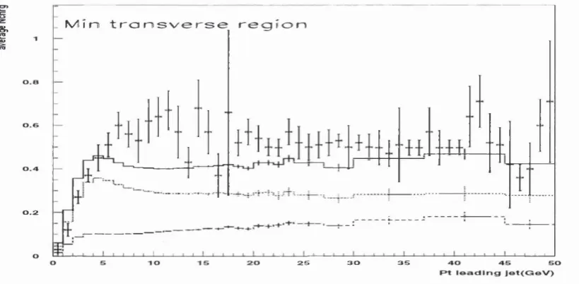
4.16 The average number of trans-Min particles as a function of Ft (leading
charged jet) in the transverse region. Solid points are the experimental CDF
data [35] and the solid line the simulated data from HERWIG 4- Underlying
Event model. Charged particles arising from the break-up of the beam and
target (dotted line) and charged particles that result from the outgoing jets
initial and final-state radiation (dotted dashed line) are shown separatly. . . 84
4.17 The average diflference, trans-Max minus trans-Min, for the number of charged
particles as a function of Ft (leading charged jet) in the transverse region.
Solid points are the experimental CDF data [35] and the solid line the sim
ulated data from HERWIG 4- Underlying Event model. Charged particles
arising from the break-up of the beam and target (dotted line), and charged
particles that result from the outgoing jets initial and final-state radiation
(dotted dashed line) are shown separately... 85
4.18 Illustration of transverse cones in the r) - (f) space with |t7 |< 1 located at the
same pseudorapidity as the leading jet but with azimuthal angle A(^ = +90°
and = —90° relative to the leading jet. Each transverse cone has an area
in ?7 - 0 space of = 0.49?r... 8 6
4.19 The average scalar pt sum of the trans-Max and trans-Min charged particles
as a function of Et (leading charged jet) in transverse cones. Solid and
hollow circles experimental CDF data [35], HERWIG + Underlying Event
model (crosses) simulated data... 87
5.1 Example of a m ultiparton scattering in pp c o llis io n ... 92
5.2 The average total number of charged particles in the event as a function of Pt
(leading charged jet). HERWIG + Hard Interaction model simulated data
(solid line ptmin = 3.0 GeV), (dotted line ptmin = 2.0 GeV), experimental
CDF data [35] (data points)... 99
5.3 The average number of charged particles as a function of Ft (leading charged
jet) in the toward region. HERWIG + Hard Interaction model simulated data
(solid line ptmin = 3.0 GeV), (dotted line ptmin = 2.0 GeV), experimental
CDF data [35] (data points)...100
5.4 The average number of charged particles as a function of Ft (leading charged
jet) in the away region. HERWIG + Hard Interaction model simulated data
(solid line ptmin = 3.0 GeV), (dotted line ptmin = 2.0 GeV), experimental
CDF data [35] (data points)...100
5.5 The average number of charged particles as a function of Ft (leading charged
jet) in the transverse region. HERWIG + Hard Interaction model simulated
data (solid lineptmin = 3.0 GeV), (dotted lineptmin = 2.0 GeV), experimental
CDF data [35] (data points)...101
List of Figures 12
5.6 The average Pt sum of charged particles as a function of Ft (leading charged
jet) in the toward region. HERWIG + Hard Interaction model simulated data
(solid line ptmin = 3.0 GeV), (dotted line ptmin = 2.0 GeV), experimental
CDF data [35] (data points)...101
5.7 The average Pt sum of charged particles as a function of Pt (leading charged
jet) in the away region. HERWIG + Hard Interaction model simulated data
(solid line ptmin = 3.0 GeV), (dotted line ptmin = 2.0 GeV), experimental
CDF data [35] (data points)... 102
5.8 The average Pt sum of charged particles as a function of Pt (leading charged
jet) in the transverse region. HERWIG + Hard Interaction model simulated
data (solid lineptrnm = 3.0 GeV), (dotted \ m e p t m i n = 2 .0 GeV), experimental
CDF data [35] (data points)... 102
5.9 The average number of the trans-Max and trans-Min charged particles as a
function of Pt (leading charged jet) in the transverse region. Solid (Max)
and hollow (Min) points experimental CDF data [35]. HERWIG Hard
Interaction model simulated data (dotted line ptmin = 2.0 GeV)... 103
5.10 The average scalar pt sum of the trans-Max and trans-Min charged particles
as a function of Pt (leading charged jet) in the transverse region. Solid
(Max) and hollow (Min) points experimental CDF data [35]. HERWIG 4-
Hard Interaction model simulated data (dotted line ptmin = 2.0 GeV). . . . 103
5.11 The average Pt sum of charged particles as a function of Pt (leading charged
jet) in the transverse region. HERWIG -f Hard Interaction model simulated
data (solid line = 2.0 GeV), (dotted line = 3.0 GeV), HERWIG
QCD hard two to two subprocess including initial and final state radiation
(solid circles ptmin = 3.0 GeV)...104
5.12 The plot of the overlap function bA{b) for two values of proton radius = 2.13GeV^
(green) and = 0.71 GeV^ (red)...105
5.13 The decrease of the proton radius by the factor of 1.73 and its effect on
the parton densities within the colliding hadrons at 6 = 0 (i.e. in a central
collision)...105
5.14 The average total number of charged particles in the event as a function of
Pt (leading charged jet). HERWIG 4- Hard Interaction model (solid line)
simulated data (with reduced proton radius), experimental CDF data [35]
(data points)...106
5.15 The average number of charged particles as a function of (leading charged
jet) in the toward region. HERWIG + Hard Interaction model (solid line)
simulated data (with ptyrim = 3 GeV and reduced proton radius), experimen
tal CDF data [35] (data points)...106
5.16 The average number of charged particles as a function of Ft (leading charged
jet) in the away region. HERWIG 4- Hard Interaction model (solid line) sim
ulated data (with = 3 GeV and reduced proton radius), experimental
CDF data [35] (data points)...107
5.17 The average number of charged particles as a function of Ft (leading charged
jet) in the transverse region. HERWIG 4- Hard Interaction model (solid line)
simulated data {with ptmin = 3 GeV and reduced proton radius), experimen
tal CDF data [35] (data points)...107
5.18 The average Ft sum of charged particles as a function of Ft (leading charged
jet) in the toward region. HERWIG 4- Hard Interaction model (solid line)
simulated data (with ptmin = 3 GeV and reduced proton radius), experimen
tal CDF data [35] (data points)...108
5.19 The average Ft sum of charged particles as a function of Ft (leading charged
jet) in the away region. HERWIG 4- Hard Interaction model (solid line) sim
ulated data {with Ptmin = 3 GeV and reduced proton radius), experimental
CDF data [35] (data points)... 108
List of Figures 14
5.20 The average Pt sum of charged particles as a function of Pt (leading charged
jet) in the transverse region. HERWIG 4- Hard Interaction model (solid line)
simulated data (withpi^nm = 3 GeV and reduced proton radius), experimen
tal CDF data [35] (data points)... 109
5.21 The average number of the trans-Max and trans-Min charged particles as a
function of Pt (leading charged jet) in the transverse region. Solid (Max)
and hollow (Min) circles experimental data, HERWIG 4- Hard Interaction
model (solid line) simulated data (with ptmin = 3 GeV and reduced proton
radius), experimental CDF data [35] (data points)...109
5.22 The average difference, trans-Max minus trans-Min, for the number of charged
particles as a function of Pt (leading charged jet) in the transverse region.
Solid points are the experimental data and the solid line the simulated data
from HERWIG 4- Hard Interaction model (solid line) simulated data (with
Ptmin = 3 GeV and reduced proton radius), experimental CDF data [35]
(data points)...1 1 0
6 .1 o’^sSpTi^pp) corresponds to a soft collision between the two soft gluons (full
color picture). Remnants are also connected to each other via t channel gluon
line...119
6.2 The soft collision between the two soft gluons, with dashed solid lines indi
cating the severed color connections between the remnants and the outgoing
gluons, forming two clusters, qiq2 and qiqô.... 119
6.3 Transverse momentum distributions of the soft (solid line) and hard (dashed
line) partons at GeV...122
6.4 Transverse momentum distributions of the soft (solid line) and hard (dashed
line) partons at ptmin=^-^ GeV... 123
6.5 Transverse momentum distributions of the soft (solid line) and hard (dashed
line) partons at Ptmm=3.0 GeV... 124
6 . 6 The average total number of charged particles in the event as a function of Pt (leading charged jet). HERWIG 4- Eikonal model simulated data ptmin, =
3.0 GeV (solid line) and 2.0 GeV (dotted line), experimental CDF data [35]
(data points)... 126
6.7 The average number of charged particles as a function of Pt (leading charged
jet) in the toward region. HERWIG 4- Eikonal model simulated data ptmin
= 3.0 GeV (solid line) and 2.0 GeV (dotted line), experimental CDF data
[35] (data points)...127
6 . 8 The average number of charged particles as a function of Pt (leading charged
jet) in the away region. HERWIG 4- Eikonal model simulated data ptmin =
3.0 GeV (solid line) and 2.0 GeV (dotted line), experimental CDF data [35]
(data points)... 127
6.9 The average number of charged particles as a function of Pt (leading charged
jet) in the transverse region. HERWIG 4- Eikonal model simulated data
Ptmin = 3.0 GeV (solid line) and 2.0 GeV (dotted line), experimental CDF
data [35] (data points)...128
6.10 The average Pt sum of charged particles as a function of Pt (leading charged
jet) in the toward region. HERWIG 4- Eikonal model simulated data ptmin
= 3.0 GeV (solid line) and 2.0 GeV (dotted line), experimental CDF data
[35] (data points)...128
6.11 The average Pt sum of charged particles as a function of Pt (leading charged
jet) in the away region, HERWIG 4- Eikonal model simulated data ptmin =
3.0 GeV (solid line) and 2.0 GeV (dotted line), experimental CDF data [35]
(data points)...129
6.12 The average total number of charged particles in the event as a function of
Pt (leading charged jet). HERWIG 4- Eikonal model, (solid line) simulated
data {ptmin = 2 .5 GeV), experimental CDF data [35] (data points)...129
List of Figures 16
6.13 The average Pt sum of charged particles as a function of Pt (leading charged
jet) in the toward region. HERWIG + Eikonal model (solid line) simulated
data {ptmin = 2.5 GeV), experimental CDF data [35] (data points)... 130
6.14 The average Pt sum of charged particles as a function of Pt (leading charged
jet) in the away region. HERWIG + Eikonal model (solid line) simulated
data {ptmin = 2.5 GeV), experimental CDF data [35] (data points)... 130
6.15 The average Pt sum of charged particles as a function of Pt (leading charged
jet) in the transverse region. HERWIG + Eikonal model (solid line) simu
lated data iptmin = 2.5 GeV), experimental CDF data [35] solid circles. . . . 131
6.16 The average number of charged particles as a function of Pt (leading charged
jet) in the transverse region. HERWIG -f Eikonal model (solid line) simu
lated data {ptmin = 2.5 GeV), experimental CDF data [35] (data points). . . 131
6.17 The average Pt sum of charged particles as a function of Pt (leading charged
jet) in the transverse region. HERWIG -f Eikonal model (solid line), HER
WIG 4- Underlying Event model (solid dashed), HERWIG Multiparton
Hard model (dotted), experimental CDF data [35] (data points)... 132
6.18 The average number of charged particles as a function of Pt (leading charged
jet) in the transverse region. HERWIG -f Eikonal model (solid line), HER
WIG 4- Underlying Event model (solid dashed), HERWIG 4- Multiparton
Hard model (dotted), experimental CDF data [35] (data points)... 133
6.19 The average Pt sum of charged particles as a function of Pt (leading charged
jet) in the transverse region. HERWIG 4- Eikonal Model for the two sets of
Ptmin = 3.0 GeV (solid line) and 2 .0 GeV (dashed), HERWIG 4- Multiparton
Hard Model ptmin = 2.0 GeV (dotted), ptmin = 3.0 GeV (dotted dashed),
experimental CDF data [35] (data points)...134
6.20 The average number of trans-Max and trans-Min charged particles as a func
tion of Pt (leading charged jet) in the transverse region. Solid (Max) and
hollow (Min) circles experimental CDF data [35], (solid line) simulated data. 135
6.21 The average scalar Ft sum of the trans-Max and trans-Min charged particles
as a function of F t (leading charged jet) in the transverse region. Solid
(Max) and hollow (Min) points are the experimental CDF data [35], (solid
line) simulated data... 135
6.22 Data on the average difference, trans-Max minus trans-Min, for the number
of charged particles as a function of F t (leading charged jet) in the transverse
region. Data points experimental CDF data [35], (solid line) simulated data. 136
6.23 The average scalar Ft sum of the trans-Max and trans-Min charged particles
as function of E t (leading charged jet) in transverse cones. Solid (Max) and
hollow (Min) circles experimental CDF data [35], HERWIG Eikonal model
(crosses) simulated data...137
6.24 The average scalar Ft sum of the trans-Max and trans-Min charged particles
as function of E t (leading charged jet) in transverse cones. Solid (Max) and
hollow (Min) circles experimental CDF data [35], HERWIG 4- Eikonal model
P t m i n = 3 GeV (solid line), HERWIG 4- Eikonal model p t m i n = 20, 40, 60,
80 GeV (dashed line) simulated data... 138
6.25 Illustration of the transverse regions in the f) - 4> space with | A(f) |< tt/2 in
the rapidity intervals 1<| Ar) |<2 on the two sides (i.e. left (L) and right (R)).140
6.26 Average transverse energy {dEt/dp) in 1 < |t7 — pjet\ <2, \(f) - <pjet\<T^/2 as
a function of the E t j e t trigger. Data points UAl at 630 GeV [39], solid line
represents HERWIG 4- Eikonal model, dashed line represents HERWIG 4-
Hard Interaction model (with reduced proton radius), dotted line represents
HERWIG 4- Hard Interaction model with P(mw=2.0 GeV... 140
List of Figures 18
6.27 The average Pt sum of charged particles as a function of Pt (leading charged
jet) in the transverse region. HERWIG + Eikonal model at -\/s = 14 TeV
(solid line), HERWIG + Eikonal model at y/s = 1.8 TeV (dashed line). . . . 141
6.28 The average number of charged particles as a function of Pt (leading charged
jet) in the transverse region. HERWIG + Eikonal model at y/s = 14 TeV
(solid line), HERWIG + Eikonal model at y/s = 1.8 TeV (dashed line). . . . 141
6.29 The average scalar Pt sum of the trans-Max and trans-Min charged particles
as a function of Pt (leading charged jet) in the transverse region. HERWIG
4- Eikonal model at y/s = 14 TeV (solid line), HERWIG 4- Eikonal model at y/s = 1.8 TeV (dashed line)... 142
6.30 The average number of trans-Max and trans-Min charged particles as a func
tion of Pt (leading charged jet) in the transverse region. HERWIG 4- Under
lying Eikonal model at y/s = 14 TeV (solid line), HERWIG 4- Eikonal model
at y/s = 1.8 TeV (dashed line)...142
6.31 Data on the average difference, trans-Max minus trans-Min, for the number
of charged particles as a function of Pt (leading charged jet) in the transverse
region. HERWIG 4- Eikonal model at y/s = 14 TeV (solid line), HERWIG
4- Eikonal model at y/s = 1.8 TeV (dashed line)...143
U N IV E R S IT Y COLLEGE L O N D O N
A B S T R A C T OF T H E S IS submitted by Ivan B orozan for the Degree of Doc
tor of Philosophy and entitled A n Eikonal M o d el for M u ltip a rticle p rod u ction
in H adron-H adron S ca tterin g
Month and Year of Submission: November 2 0 0 2
The purpose of this thesis is the introduction of a model for multiparticle pro
duction in hadron-hadron interactions.
An introduction to the broad issue of perturbative Quantum Chromodynamics
(QCD) is presented in the first chapter with special emphasis on the concepts of renor
malization, asymptotic freedom and scaling violation. In addition non-perturbative
concepts such as Regge theory and Regge pole param etrisation of the total cross sec
tion are mentioned.
The second chapter is a broad introduction to the Monte Carlo techniques used
in event generators and numerical integrators with special emphasis on the methods
used in the HERWIG event generator.
The third chapter contains a brief overview of the main physics and methods
used in HERWIG for simulation of large momentum transfer collisions between two
A bstract 20
hadrons.
In Chapter 4 we introduce the physics of the underlying event and adopt a sim
ple jet definition used by the CDF collaboration in the analysis of charged particle
component of jets simulated by HERWIG in three different topological regions. For
hard scattering proton-antiproton collisions we simulate the underlying event activ
ity in each region using HERWIG’s Underlying Event model and compare it to the
experimental data. We thus independently confirm results obtained by the CDF col
laboration.
In Chapter 5 we present the M ultiparton Interaction model used as a substitute
to the HERWIG Soft Underlying event model. We examine whether the addition of
secondary hard scatters to the main hard interaction improves the simulated data on
the underlying event. We propose to tune the value of the proton radius used in the
Hard M ultiparton Interaction model in order to obtain a good agreement with the
experimental data.
In Chapter 6 we introduce a new Eikonal Monte Carlo model in order to simulate
m ultiparticle production in hadron-hadron interactions. The model contains a single
phenomenological input the total cross section for pp and pp scattering. We show a
broad agreement between our model predictions and experimental data. We discuss
its main advantages over the two underlying event models used in chapters 4 and 5.
Finally we use the new Eikonal model to predict the underlying event activity which
should be expected at the LHC.
No portion of the work referred to in this thesis has been
subm itted in support of an application for another degree
or qualification of this or any other university or other
institution of learning.
D ed ica tio n
Dedicated to the memory of
Prof. Dragoljub Mihailovic
(1917 - 1994)
“...Iko m oja diko”
I would first like to express my infinite gratitude to my grand-father for his encour
agement and material help without which probably nothing of my initial resolve to
study physics would have been realized and to CCLRC for funding my postgraduate
studies.
My big thank goes to my family for all the love you have given to me (particularly
to my mother Alexandra and my sister Maria).
During these three years of my PhD I have had the opportunity to work within
three different research groups, I joined the HEP group of the University College
London in October 1999 and started my work under the supervision of Dr. Jon
Butterw orth, who has introduced me to the interesting problem of the underlying
event in lepton-hadron and hadron-hadron collisions, thanks Jon for all your help and
encouragement.
After my first year at University College London I have moved and joined the
RAL theory particle physics group under the supervision of Dr. Michael Seymour,
Mike thank you for all your help, patience, encouragement and invaluable discussions
during these past three years.
My special thank goes to Dr. Jeff Forshaw for his help and useful discussions and
the Manchester Theory group for their hospitality and support during the final year
of my thesis.
Thank you Alberto Ribon and Kosuke Odagiri for all your help and friendship.
Acknowledgements 24
Thank you Dr. Chan Hong-Mo for all the interesting discussions and encourage
ment during my stay at RAL.
My special thanks go to Dr. W.G Scott and Prof. Ken Peach for their help
and Prof. R.G Roberts and Prof. Frank Close for making my stay at RAL such an
interesting experience.
Finally thanks to all my fellow students at UCL: particularly to Claire Gwenlan,
Chris Smith and Richard Steward and Greg Moley for the help during my stay at
RAL.
Ivan Borozan graduated with an MSci in physics from University Col
lege London. In September 1999 he started this thesis at the De
partm ent of Physics and Astronomy as a member of the High Energy
Physics Group of University College London.
“It is not certain that everything is uncertain.”
Blaise Pascal
C hapter 1
In trod u ction
1.1
Introduction
In this chapter we present a brief overview of the main concepts used in Quantum
Chromo Dynamics, the theory of strong interactions. Most of the concepts presented in
the following sections are implemented in the HERWIG Monte Carlo Event generator,
our principal tool for data simulation. Furthermore in this thesis we will propose
and use a new model with HERWIG as its kernel. Thus it is essential th a t the main
concepts and approximations used in HERWIG (as a “faithful” representation of the
perturbative QCD part) are transparent to anyone who is going to use it. W hat are
the advantages of using a Monte Carlo event generator in our simulations ? First it
is particularly suitable for describing complex final states th a t traditional analytical
techniques are not capable of, second it is particularly convenient since we can impose
on our final states the same experimental cuts as those used in the experiment. Thus a
Monte Carlo event generator is an interesting tool th at is particularly im portant if we
are to estimate the accuracy of perturbative QCD predictions in this particular case,
or more generally to simulate the physics of the Standard Model as a background to
some new physics.
The structure of this thesis is as follows: in Chapter 2 we present an overview of
the most im portant Monte Carlo techniques used in Monte Carlo event generators, in
Chapter 3 we describe the main assumptions and approximations used in HERWIG
for simulating two-to-two parton-parton scattering, in Chapter 4 we compare d ata
simulated with HERWIG QCD Monte Carlo event generator to those of experimen
tal proton-antiproton collisions at 1.8 TeV involving a hard scattering and focus on
whether our ‘default’, Monte Carlo model describes correctly the ‘underlying event’ in
hard jets. In Chapter 5 we present an overview of the Hard M ultiparton interaction
model and examine whether this alternative model describes b etter the ‘underlying
event’. In Chapter 6 we propose a new model for simulating the ‘underlying event’
based on an eikonal approach and compare it to HERWIG’s default Underlying Event
model and the Hard M ultiparton Interaction model results. Finally we test the pre
dictability of our model by comparing our simulated d a ta to the experimental U A l
Chapter 1. Introduction 28
measurement at -^5=630 GeV.
1.2
QCD
The theoretical and experimental study at high energies of hadron-hadron, lepton-
lepton and lepton-hadron interactions has led to a description of properties of the
strong force. The strong force is one of the four fundamental forces in nature and
is responsible for nuclear binding and hadron-hadron interactions. Quantum Chromo
Dynamics (QCD) is considered today as the most correct theoretical description of
strong interactions.
The QCD Lagrangian is formulated in terms of its fundamental fields, quarks and
gluons. Each fundamental particle of QCD carries, together with the usual quantum
numbers an additional degree of freedom, named colour. Colour was introduced to
explain the wave function for the doubly charged A++ baryon, having the spin of 3/2.
If we are to construct a A++ wave function, using three identical quarks in their ground
state, we will obtain a symmetrical wave function of space, spin and fiavour SU(3)/
degrees of freedom. However as quarks have spin 1/2, Fermi-Dirac Statistics dictates a
totally anti-symmetric wave function for the A++ baryon. By adding the colour degree
of freedom (with three possible values) to quarks, the A++ baryon wave function can
be made totally anti-symmetric in colour. The elementary fundamental particles of
QCD cannot be observed in experiments as such, only their bound states, such as
hadrons are. QCD in consequence exhibits a particular behaviour, at small distances
the fundamental particles can be essentially considered as free (i.e small coupling
constant) and at large distances (% 1/m) and large coupling constant, quarks and
gluons form bound states. The decrease of the coupling constant at small distances
is known as asymptotic freedom and the mechanism forcing quarks and gluons into
asymptotic states is known as confinement. Furthermore because coloured states are
not detected in experiments, one additional constraint is required, th a t only colour
singlet states can exist in nature. The behaviour of the coupling constant at large
distances prevents perturbative QCD calculations from predicting asymptotic final
states.
The idea of colour was checked in early experimental tests, for example the rate
of decay tt® —> 7 7 or the ratio of the e+e" hadronic total cross section to the cross
section for the production of a muon pair. The evidence for the existence of approxi
mately point-like particles was provided by the early electron deep inelastic scattering
experiment at SLAC showing the scaling behaviour of the measured cross section.
The point-like particles inside hadrons were term ed partons and identified later with
quarks and gluons.
1.2.1
Q CD Lagrangian
The expression for the QCD Lagrangian density, invariant under SU(3) local gauge
phase transform ations, can be written as
^ — ~ ~ + ^ gau ge fixing + ^ g h o st- ( l - l )
f ^
The quark and gluon fields are represented by -0 and A respectively. T> is the
covariant derivative {V^)ab = d^ôab + ig{t^A^)ab acting on triplet quark fields and
{Pii)ab = df^ÔAB + ig{T^A^)AB on octet gluon fields. The flavour number, / in eq.1.1,
runs over all n / quark flavours. is the field strength tensor derived from the gluon
field
= d X - (1.2)
The indices A, B, C run over 1,..., — 1 colour degrees of freedom of the gluon field
and a, 6, c run over the triplet representation of the colour group, are the S U (Ne)
group structure constants, g is the coupling constant which determines the strength
of the interaction between the coloured quanta and Nc is the number of colours in the
theory. We m ention here, without going into further details, th at the choice of gauge is
Chapter 1. Introduction 30
necessary for defining the gluon propagator and the ghost term cancel the unphysical
degrees of freedom which would otherwise propagate in the covariant gauges.
1.2.2
R en orm alization
Feynman rules can be directly deduced from the Lagrangian in eq.1.1. At higher
orders, divergences will appear in loop integrals, when the momentum in the loop
integral goes to infinity (ultra-violet divergences) or when the outgoing partons are in
the soft or collinear lim it (infra-red divergences). In the case of infrared divergences
the loop and soft and collinear contributions cancel each other*, making their sum ’in
frared’ finite. However for loop integrals such as shown in fig. 1.1, the infinite integrals
need first to be regularized before the infinite (ultra-violet) divergences are absorbed.
One way to regularize an infinite integral would be to introduce a momentum cutoff
and then absorb the divergent term into newly redefined fields or parameters. The re
definition of the fields and parameters after absorption of the divergent term is known
as renormalization. We give here an outline of the renormalization of the bare strong
coupling g (for more details see [3]).
If we are to compute the effective strong coupling at one loop level we would get
+ 0(^^), (1.3)
g3
9 e f f — 9 e f f { Q ) — 9
3 2 ^ ^
where A is the ultraviolet cutoff, for A—>-oo, ^e//(Q^) is divergent (i.e. ^e//(Q^)~>oo).
The procedure now consists of introducing a renormalization scale at which the
renormalized coupling (as opposed to bare) for some choice of will be fixed
to a particular finite value. The new effective (measured) coupling 9eff{Q‘^) becomes
then a function of the renormalization scale fj? and can be expressed as
Q'
9 e f f { Q ‘^) 9 e f f { l J ' ‘^)
-An often used m ethod for regularizing infinite integrals is dimensional regular
ization. The idea is th a t the loop integral is only divergent in four dimensions, for *Initial-state collinear divergencies do not cancel but can be factorised and replaced by non-perturbative parton distribution functions
smaller number of dimensions the integral is finite. Thus by integrating in D = 4-e (e
> 0) dimension a finite result should be found. The one-loop contributions shown in
fig. 1.1, contain respectively integrals of the form [1]
T _ Ç _____
^ J {27ry {k“^ — m ^ ) { { k q y — m'^)^
2 (27T)4 g)2' I
'■ = / ( # # ' ( " )
r
F
„
^ “ J (27r)'‘ A:2(fc + g)2' ^ ' ■'
For an expression with two factors in the denominator we first introduce Feynmann
param eters x and y defined as
J
b= I !
+ T - x)B)2 = r
+
M +
y s r
(19)
We can now express eqs.1.5-1.8 respectively as
(119)
^
lo
‘^"'/'^^(27r)^{/2-A)2’
(^'^^)
h = I ( P _ A )2’ (1-1 2)
% '^^/‘^'(27
t)4 (P -A )2 ’
(^'^^)
where I = k xq^ A' = — x { l — x)q‘^ and A = —x{l — x)q^.
We perform the Wick rotation of the variable I and define the Euclidean 4-
momentum variable Ie as
y — il%, 1 = Ie- (1.14)
The integrals from eqs.1.10-1.13 can now be evaluated in four-dimensional spherical
coordinates using the general expression
L
(i| +A)2’
(^-^5)
Chapter 1. Introduction 32
b)
c)
k2T2 0r
Figure 1.1: One loop Feynman diagrams.
which is badly ultraviolet divergent. This integral can however be regularized using
dimensional regularization.
In d dimensions the integral in eq.1.15 can be w ritten as [1]
Defining e = 4 — d, near d = 4 we use the approximation,
r
(2 - ^ ) =r
( I ) = 1 + 7E + 0(e), (1.17)where 'Je ~ .5772 is the Euler constant and the integral in eq.1.16 becomes then for
d ^ 4
^ ^ ( 4 ^ ( ! " + k^(4%0 + 0 ( e )) (1.18)
The divergence in the loop integral now shows as a pole in e. The pole in e can
be removed by adding counter terms to the Lagrangian and re-interpreting the new
terms as the renormalized fields and coupling. If the counter terms exactly cancel the
e pole then this defines the minimal subtraction scheme {MS). However if additional
constant terms (such as — log (4%)) are also removed then this defines a modified
M S scheme known as M S . One drawback of the dimensional regularization is th a t the
coupling being dimensionless in d= 4 acquires dimensions in d 4 and the subtraction
scale /i is introduced and factors of keep appearing.
1.2.3
A sy m p totic freedom
A physical observable should not depend on the choice of the renormalization scale.
This statem ent can be formulated as the renormalization group equation (RGE) (see
for example [2]),
d 2 d odas d
5/i^ d a
where 0(Q^//u^, as) is a dimensionless physical observable with physical scale The
expression in eq.1.19 can be rewritten as
0 (e)[p (Z),(%g) == 0, (1.2 0)
dt das
where the variables t and ^{as) are defined as
t = l n ( — V /3{as) = (1-2 1)
The first order differential equation in eq.1 .2 0 can be solved by defining the running
coupling CKa(Q^) as
t = / = a,. (1.2 2)
Jas P\^)
By differentiating eq.1.22 we can check th at
231
dt
and th a t 0 (1, is a solution of eq.1.2 0.
The running of the coupling constant as is thus determined by the RGE
= (1 24)
Chapter 1. Introduction 34
In QCD, piag) in eq.1.20, can be expanded pertubatively [2] as
^{pcs) = —6cKg (1 + y ocg + 0(q'^)). (1.25)
At one loop level, graphs from fig.l.l.(a,b) are used to obtain the value of hwhich
can be expressed as [2]
^ l i e A - 2uf ^ (33 - 2nf)
1271- 127T ■ ^ ’
At higher order h' is calculated to be [2]
, _ (17C^ - bCAUf - ZCpUf) _ (153 — 19u/)
27r(llC^ - 2rif) ~ 27t(33 - 2uf) ' ^ ^
If higher order terms to one loop level in eq.1.25 are neglected, eq.1.24 can be rewritten
as
Q 2 9 2 0 1 _ (1.28)
which gives as solution
“ 1
+
( ^ 0 ■The role of the running coupling ag(Q^) in eq.1.29 can be seen as twofold, first it
compensate for the Q[Q'^/ dependence of the renormalization scale /i, second
it regulates the 0(Q ^//i^, «5), scale dependence. From eq.1.29 we notice th a t the
running coupling ag(Q^) decreases and tends to zero as Q (i.e. t) increases. This
property of QCD is known as asymptotic freedom.
The renormalization scale p can be removed from the running coupling by intro
ducing a scale Kqcd at which the coupling will diverge (i.e. as will become strong)
by setting [2]
In
AgcD Joca{Q'^) P{u)
The integral in eq.1.30, at one loop level, leads to [2],
-- 6ln (QS/A&ca) '
where Aqcd is of the order of 200 MeV and indicates the boundary for Q % iGeV
below which becomes large and perturbative calculations break down. The
value of Aqcd is determined from the measurement of and will depend on the
number of flavours used in loop calculations and the renormalization scheme. The
often used value of Aqcd is the 5-flavour QCD scale performed in the modified
minimal subtraction scheme [4]. In fig.1.2 we show various experimental tests of the
running coupling in good agreement with the theoretical predictions. The average
0.3
0.2
0.1
Theory
Data 1 i J l
Deep b'-elasiic Seau.enng AnnihlWiun
Hadron Collisions I h avy yu'irkonia
...& ...
' o : o
# 8*
ots(Mz) 251 MeV~— 0T215 213 MeV
178 MeV
<1.1184 0:1153
^
Q[GeV]
Figure 1.2: Experimental tests of the QCD running coupling [5].
world value for the coupling constant at the mass is
a,(M z) = 0.118 ± 0.0 0 2, (1.32)
Chapter 1. Introduction 36
from which the value of can be deduced to be
= 2 0 8 lg MeV. (1.33)
1.2.4
T he proton structure and th e naive parton m od el
The information about the proton structure is extracted from deep inelastic lepton-
hadron scattering (DIS) experiments. The two incoming particles (usually electron and
proton), shown in fig.1.3, are pictured as exchanging a virtual photon (or boson)
with large transverse momentum squared during which the proton breaks down into
a struck quark and remnant jets of hadrons.
P
Figure 1.3: Illustration of an DIS collision.
In fig.1.3 the incoming and outgoing lepton (electron) four-momenta are labeled
and the incoming hadron (proton) four momentum as and the momentum
transfer as qi^ = k^ — k'^. The standard deep inelastic variables can be defined as
u = p - q ,
The inclusive spin averaged cross section for lepton-hadron scattering can be
w ritten as
\xy^F,{x,Q^) + { l - y ) F ^ { x , Q ^ ) ] , (1.35)
dxdQ"^ xQ^
-in which the mass of the proton can be neglected and where is the electromagnetic
coupling constant. In eq.1.35 Fi and F2 are gauge invariant functions called structure
functions parametrizing the structure of the hadron probed by the virtual photon. In
the leading order perturbative QCD picture the photon is considered to scatter from
a point-like constituent of the proton moving parallel to it and carrying a fraction e of
the proton momentum. At leading order (7*^ —> q) the form of the structure functions
is given by
2Fi(x, = - F2{x, = (1.36)
X g .'O g
where q{x) is a quark momentum distribution which describes the probability th at the
struck quark carries a fraction x of the proton’s momentum p. Thus at the leading
order the structure functions depend only on x; this is known as B jo r ke n scaling (i.e.
partons behave as point-like particles) as shown in Fig. 1.4. The relation between both
structure functions is known as the Callan — Gross relation and is the consequence
of quarks being spin 1 / 2 particles.
1.2.5
Scaling violation and th e A ltarelli-P arisi equations
In this section we show how QCD gluon radiation introduces a dependence of the
F2 structure function.
Adding next to the leading order terms {'y*q -4- qg) to the leading order {'y*q -4 q)
as shown in fig. 1.5 the F2 structure function is modified to
Chapter 1. Introduction 38
O’
Q [GeV"]
1000
Figure 1.4: Scaling of the F2 structure function taken from [2]
1 1 4- 2% 4- 2(22) - t l - z
where the quark momentum fraction is expressed as
X O'
(1 - J
Q '
(1.38) e 2pi-q {{pi + q f - q^) s + Q'^’
and variables with a hat indicate th a t we are considering a process at the partonic
level and x is the usual Bjorken variable.
The expression in eq.1.37 has two singularities. The first singularity arises when
2 —)• 1 and corresponds to the limit
(1.39)
This singularity is known as infrared soft and corresponds to the em itted gluon with
momentum k = 0. We will explain how the soft infrared singularity cancels with loop
vertex corrections, for now we regularize it with a cutoff at Zsoft< 1
/emu
Figure 1.5: Real part of the NLO contribution to 7*g —> q.
The second singularity in eq.1.37 arises as f 0 and is known as the mass
or collinear singularity. The collinear singularity corresponds to the incident quark
em itting a collinear gluon while itself remaining on the mass shell. We regularize the
collinear singularity with a cut off at f which will be absorbed into the bare
quark distribution. Keeping only leading logarithms, the F2 structure function can
now be expressed as
,2^, / /-)2
q ~ \/^ c o ll,
We can chose to set equal to the renormalization scale /i^ at which the coupling
as is defined, and express F2 as
q^) = E 4 ,(z ) + E ^
X g g Z7T
where Pgg represents the probability.
P q q = C l
1 4- 2%
1 - 2 (1.42)
of a quark to emit a gluon with a momentum fraction 1 — 2, and where the colour
factor Cf —
At this point we introduce virtual gluon corrections to the leading order 7*g —> q
process as shown in fig. 1.6.
The sum of the amplitudes squared of fig. 1.5 and fig. 1 .6 leads F2 to be expressed
as
(1.43)
Chapter 1. Introduction 40
+
Figure 1.6: Virtual part of the NLO contribution to 7*g —> q.
In eq.1.43 the soft singularities have been canceled by the virtual corrections to 7*g —>
q process, in doing so the splitting function Pqq has been modified and now includes a
term which removes its original singularity. Pqq can now be expressed as
where the (+) prescription is defined as
p . . / w _ / " . . / w - / ( i )
Jo
(1.44)
, dz ^ =
f
dz-' 0 (1 — z)_|_ Jo 1 — z (1.45)
In eq.1.43 in addition to the x dependence, the structure function now has a
logarithmic dependence which violates Bjorken scaling with /i the cutoff scale for
collinear gluon emissions. The logarithmic dependence can be absorbed into the
quark probability distribution function and eq.1.43 can be rewritten as
- F 2 (x, Q ‘^) — 53^ 9 / — (^(^) + A g(e, ^1 - - 'j
g * ' X £ ^ \ C /
(1.46)
where
r d e
ZTT
(^)
L(i)
•From eq.1.47 the quark density q(x,Q'^) now depend on and its evolution as
function of can be written as
d
q2) _ £ y g (6, Q ^)P „ g ) , (1.48)
d In ^ ^ ' 27T
The expression in eq.1.48 is the direct consequence of quarks interacting through the
gluonic field. As the scale of photon-quark interaction increases, the number of partons
sharing the proton m omentum is increased and so the probability of finding a quark at
small X, Furthermore because high-momentum quarks lose momentum through gluon
radiation the chance of finding a quark with high x should decrease.
To the diagram in fig. 1.5 we should also add contributions from the gluon anni
hilation process (7*^ —> qq) shown in fig. 1.7. The F2 structure function contains thus
qbar
qbar
Figure 1.7: NLO contribution from gluon annihilation.
an additional contribution
where g{s) is the gluon density in the proton and where
X
- + 1-
-X
\ e
is the probability for a gluon to annihilate into a qq pair.
The complete quark evolution equation can now be w ritten as
d
^ L e ( g ) +9{^>Q^)F<i9 ( ^ ) ) . (1-51)
for each quark flavour / and is valid for any massless quark and antiquark. The full
expression in eq.1.51 is known as Dokshitzer-Gribov-Lipatov-Altarelli-Parisi (DGLAP)
[6, 7, 8, 9] equation. The DGLAP equation describes a quark with momentum fraction
Xcoming from a parent quark with larger momentum fraction e which has radiated a
gluon. The corresponding equation for the gluon distribution can be written as (1.50)
d
9(x,Q ") = { f ) + 9{e,Q^)P,ç ( f ) ) , (1.52)
C hapter 1. Introduction 42
where
and
Pgg
=
2C
a\
--- h
z { l - z ) ] + 27t6 (^(1 - z),(1.53)
(1.54) \ ^ (1 — ^)+ /
are respectively the gluon-quark and gluon-gluon splitting functions, and where b is
given in eq.1.26. In fig.1.8 we show d ata on the structure function and prediction
from the DGLAP evolution equations using MRS [10] parton distribution function set.
.6
.5
.4 —
1---1---1—r-TTTT
x=0.0125 x= 0.0175 x=0.025 x=0.035 x=0.05 x=0.07 x=0.1
1 I I I I I I
Fr
• NMC.4 t
-::g
.5 rr
.45 p .4 p .35
L-.35
I
— x=O.10
o BCDMS (x0.9B)
--- MRS(A)
f
- u U t o p 4
à
-i 0 o n
*- 4 - n^o u u
[GeV]
3
x = 0.225
x=0.275 x=0.35 x=0.45 x=0.55 x=0.65 x=0.75
Figure 1.8: QCD fits to muon-proton DIS F2 taken from [2]
1.2.6
P arton d istrib ution functions
Parton distribution functions are obtained from accurate measurements of the struc
ture functions ^2(0:, The procedure consists of performing a QCD fit to the entire
experimental d a ta set. The QCD fit starts by assuming a certain param etrized form in
X for the different parton distribution at low parton distributions are then evolved
up in with a particular value of through the DGLAP evolution equations to
the values of where the structure function has been measured. The initial set of
parameters is then chosen to correspond to the best fit to the experimental data. In
fig. 1.9 we show a set of parton distribution functions at = 20 GeV^.
Chapter 1. Introduction 44
2
= 20 GeV M RST partons
1.5
><
X
1
g /i o
0.5
0
10
Figure 1.9: Parton density distributions as functions of x for = 20 GeV^ taken from [1 1].
1.3
R egge Theory and Total cross sections
1.3.1
Two b ody scattering
In this section we give a brief overview of the concepts th at we use to derive the
remarkable unitarity relation called the “optical theorem” . In fig. 1.10 we show the
general expression for two-to-two particle scattering processes. The scattering process
s
Figure 1.10: The scattering process in the s channel of eq.1.55.
between two particles in the s channel can be w ritten as
a(pi) + b{p2) c(j>3) + d{pi), (1.55)
where pi (2=1,...4) are the respective 4 momenta of particles a, b, c and d. The Mandel
stam variables s, t, n, which are invariant under Lorentz transformations, are defined
as
s = (pi-\-p2f,
t = (Pi
U = { p i - P 4 )^ .
For massive particles the Mandelstam variables satisfy the relation
4
5 + t + u =
(1.56)
(1.57)
(1.58)
(1.59)
which leaves us with only two independent variables which we choose to be s and t.
For the s-channel process t represents the momentum transferred and the scattering
angle between particles 1 and 3 can be expressed as
t = m l + m l - 2pip3,
= TTii-1- m3 - 2E i^ 3 + 2|p i ||p3| cos (^).
Thus for an elastic process
^ (P i) + Kp^) —^ ^ (p i) 4- 6(^2),
(1.60)
(1.61)
(1.62)
Chapter 1. Introduction 46
in the forward direction (i.e. ^ = 0) it is zero.
The scattering process in eq.1.55, and hence its scattering am plitude Aab, should
be Lorentz invariant, thus the scattering am plitude can be expressed as a function of
the Mandelstam variables s and t.
The differential cross section for the process in eq.1.55 can be expressed as
da = (1,63)
r
where F is the flux of the incoming particles and dQ is the Lorentz invariant phase
space factor which for two body scattering is given by
dQ = (27r)^5<^) (P3 + P 4 - P I - P 2 ) ( 2 ^ ) ^ E 4 ’
where free particles are represented by plane waves with the normalization of 2E
particles per unit volume. We express the flux factor F in eq.1.63 as
F = 4^[(piP2)^ - (1.65)
which in the high energy limit becomes F % 2s.
In the center-of-mass frame where |pi| = |p2 | and [pg] = |p4 | the differential
cross section is expressed as
da 1 IpsI
dücm 647T^S |pi| where for spinless particles
(1.66)
dÇlam = d{cOS {9))d(t) = - r - ^ (1. 67)
^iPillPal
The Lorentz invariant expression in eq.1.66 can now be expressed as
da 1
dt IbTTS^\Aab{s,t)\ • (1.6 8)
1.3.2
T he S-m atrix, u nitarity and th e op tical theorem
The scattering operator S is such th a t its m atrix elements between the initial and final
states { / I 5 I i) squared give us the probability Pfi th a t | / ) will be the final state
resulting from | i) i.e.
Pf i =1 { / I 5 I i> P = (i I 5 t I / ) ( / \ S \ i ) , (1 .6 9 )
where is the Herm itian adjoint of S. The S — m at rix can be expressed as the sum
of two parts, the non-interaction part (the identity operator) and the interaction part
(containing the dynamics of strong interactions)
Sfi = Sfi -f iTfi. (1.70)
For strong interactions with high momentum transfer the scattering m atrix elements
can be calculated using standard perturbative QCD techniques where the T — matrix
is usually defined as
{ f \ i T \ i ) = i { 2 - K f S ^ ^ \ ' £ p f - (1.71)
and where A f i is th e scattering amplitude for the state | i) to end in the state | / ) .
The S — m a tr ix contains the following assumptions:
Postulate{i)
The scattering process and hence the S — mat rix is Lorentz invariant.
Postulate{ii)
The scattering S — m a t r ix is unitary. By using the conservation of probability, if we
are to start with some initial state | i) the probability th a t there will be some final
state I / ) must be unity. From eq.1.69 this translate to
^ ^ I I S' I 2) \^= I 5^ I n )(n I 5 I z)
n n n
= (i I S ' S I i), (1 .7 2 )
where free particle states | n), constitute a complete orthonormal set of basis states
satisfying the completeness relation,
E I 1 = 1 (1.73)
n
Since eq.1.73 m ust be true for any state | z) we have
S^S = l = S S l (1.74)
![Figure 1.2: Experimental tests of the QCD running coupling [5].](https://thumb-us.123doks.com/thumbv2/123dok_us/8213890.1372669/36.595.122.514.263.639/figure-experimental-tests-qcd-running-coupling.webp)
![Figure 4.17: The average difference, trans-Max minus trans-Min, for the number of charged are the experimental CDF data [35] and the solid line the simulated data from HERWIGparticles as a function of Pttarget (dotted line), and charged particles that resu](https://thumb-us.123doks.com/thumbv2/123dok_us/8213890.1372669/101.595.68.515.49.493/average-difference-experimental-simulated-herwigparticles-function-pttarget-particles.webp)