Removal of Pollutants by Gravitational Settling on the Pollutant Distribution Emitted from the Line Source

(1)

Removal Of Pollutants By Gravitational Settling On

The Pollutant Distribution Emitted From The Line

Source

KRISHNA S Government Independent PU

College Bharathinagara, Mandya (Dist.)– 571422,

Karnataka, India. Email – [email protected]

LAKSHMINARAYANACHARI K Department of Mathematics, Sai Vidya Institute of Technology, Raj

anukunte, Bangalore – 560 064, Karnataka, India. Email –

[email protected]

PANDURANGAPPA C Department of Mathematics, University B. D. T. College of

Engineering, VTU, Davanagere – 577004,

Karnataka, India. Email –

[email protected]

ABSTRACT

A comprehensive two-dimensional mathematical model of secondary in addition to primary pollutants is presented. The model considers the pollutants dispersion emitted from line source to investigate the effect of removal of larger pollutants because of gravitational acceleration. The realistic wind velocity and eddy diffusivity profiles are considered in the model. The intricate problem is solved numerically using Crank-Nicolson finite difference technique. As gravitational settling velocity rises the concentration of secondary pollutants reduces everywhere.

Keywords— Mathematical model, Line Source, Air Pollutants, Gravitational settling, Finite difference method.

I. INTRODUCTION

Globally air pollution is one among the major problems and has become a serious threat as its effect on living system and its environment is highly unendurable. Due to radical increase in number of industries and vehicles running on the road, the grown cities are on the front to suffer from the pollutants effect. For instance, recently in the month of November 2017 in Indian city New Delhi, a series of vehicles collide one on the other continuously in a highway road as fog is covered the entire city and couldn’t even able to see the things which are 10meters apart. As a result the government ordered to take out own vehicles only on odd days to control the vehicular emission to the atmosphere. In the same time and city the SriLankan cricketers came out to the field with a mask covering their nose and mouth to avoid pollution in the test cricket match against India, which is the first time in cricket history that cricketers wearing air filters and playing. And some of SriLankan cricketers struggled with bad health conditions. The increasing levels of air pollutants emitted from motor vehicles results partly in rising trends of asthma. The increasing prevalence of asthma is associated with a rapid growth in the number of motor vehicles that are in use [1]. Many studies have shown that the contribution of vehicular exhausts on the human health is considerable in grown cities [2].

There are studies related to vehicular emissions dispersion [3-5] which are analytical in nature and studied the advection diffusion equation for the atmospheric dispersion of pollutants originated from a line source. These studies did not consider the effect of chemical reaction of pollutants in the atmosphere. There is a time dependent model [6] of air pollution which considers the effect of chemical reaction of air pollutants and variable profiles of wind velocity and eddy diffusivity. However the source here is an area source. All the above models are left out the mesoscale wind effect on pollutants. There is a model [7] which includes the mesoscale wind effect on the pollutants and their chemical reaction in the air for pollutants emitted from line source. This study not considered the effect of removal of pollutants. There is a mathematical model [8] with time dependency of primary pollutants and their secondary product which considers the removal by settling of pollutants. This model is an area source model and mesoscale effect is not included. Pandurangappa C, et al. [9] developed a study for pollutant distribution considering all the effects of mesoscale wind, chemical reaction and removal of pollutants but for an area source.

(2)

diffusivity are used here. We employ the finite difference technique by Crank-Nicolson to solve the problem numerically. Here the solution describes the concentration of line source pollutants downwind of an infinite crosswind on the ground.

II. MODEL DEVELOPMENT

The physical layout of the problem consists with finite downwind distance and infinite crosswind dimension of an infinite crosswind line source on the ground. Pollutants are assumed to be transported horizontally in perpendicular direction by a large-scale wind and horizontally as well as vertically by a local wind called mesoscale wind. Large-scale wind is a function of vertical height (z) and local wind is a function of both height (z) and distance (x). Mesoscale wind is produced due to urban heat island. The center of the city i. e.,

x



l

2

is considered as the center of heat island, where

l

is the length of the city. We have taken the city length in this problem as

l



6

km

and the concentration of pollutants is calculated in the region

0

 

x

l

. The line source of pollutants is kept at

x



0

, that is at the beginning of the city. We have considered chemically reactive pollutants and are transformed into secondary pollutants through first order chemical reaction. The description of physical layout of this problem is as shown in the figure1.

Figure 1: Physical layout of the model.

The advection diffusion equation for general species of air pollution is given by

x y z

C

U

V

W

K

kC

t

x

y

z

x

y

z

















































































(1)

where

C

is the concentration of pollutants at any location



x y z

, ,



and time

t

,

U

,

V

and

W

are the velocity components along

x

,

y

and

z

directions respectively,

K

_x,

K

_yand

K

_zare the eddy – diffusivity coefficients along

x

,

y

and

z

directions respectively and

k

is the first order chemical reaction rate coefficient.

Now the following assumptions were formulated  Pollutants are chemically reactive.

 The velocity of wind along the x direction is so large that the x direction diffusion is neglected.

 Along crosswind direction the lateral flux of pollutants is assumed to be small i.e.,

0 and

_y

0.

C

V

K

y

























A. Primary Pollutant

(3)

along horizontal and vertical direction and

W z

( )

denotes the velocity in the vertical direction because of the effect of mesoscale wind.

B. Initial and boundary conditions of Primary pollutants

We presume that the region considered is pollution free at the beginning of the emission. Hence the initial condition is given as:

0, at

0, 0

and 0



 

p

C

t

x

l

z

H

(3)

Also we assumed that no background pollution is entering the region of interest at x=0, i.e.,

0, at

0, 0

and t > 0



 



p

C

x

z

H

(4) The boundary condition for a continuous line source located at origin of strength Q (in the z-direction which has an infinitesimally small extension) is as follows (W Koch [3]):

 

At the ground, we assume there is no transfer or deposition of pollutants. Thus there is no concentration gradient at the ground level i.e.,

The pollutants considered are confined inside the mixing height and no leakage across the top boundary of the mixing layer. Therefore we have:

0, at

, 0

and

0

The basic governing equation (1) under the above formulations for secondary pollutant is given as

( , )

( )

D. Initial and boundary conditions of Secondary pollutants

We assume that at the beginning of the emission the region considered is pollution free. Therefore we get initial condition as:

0, at

0, 0

and 0



 

s

C

t

x

l

z

H

(9)

We presume that no background pollution is entering the region of interest at x=0, i.e.,

0, at

0, 0

and t > 0



 



s

C

x

z

H

(10) At the ground, we assume there is no transfer or deposition of pollutants. Thus there is no concentration gradient at the ground level i.e.,

The pollutants considered here are confined inside the mixing height and across the top boundary of the mixing layer there is no leakage. Therefore we have:

(4)

stability length, friction velocity, net heat flux etc., are considered in accordance with Pandurangappa C [10] are used to solve the equations (2) and (8).

For neutral atmospheric condition of stability the surface layer is assumed to be terminates at



*



0.1

/

z



k u

f

and for stable atmospheric condition of stability the surface layer extended up to

z



6

L

,

where

k



0.4

is the Karman’s constant,

u

_* is the friction velocity,

f

is the Coriolis parameter and

L

is the Monin-Obukhov stability length parameter.

For neutral atmospheric condition of stability the following wind velocity profiles are used

 

*





0

For stable atmospheric stability condition the wind velocity profiles used are

 

*





0





atmospheric condition of stability above the

surface layer (planetary boundary layer) the wind profiles used are

 

,







0





1



0



For both surface and planetary boundary layer the eddy diffusivity profiles used are

(5)

IV. METHOD OF SOLUTION

The objective of this mathematical model is to study and examine the concentration of primary pollutants which are chemically reactive and their secondary products emitted from a line source with mesoscale type wind. For this we need to solve equation (2) with initial and boundary conditions (3) to (7), and equation (8) with initial and boundary conditions (9) to (12). It is tedious to obtain the analytical solutions of (2) and (8) due to the variable wind speed and diffusivity forms. Thus we have used Crank-Nicolson finite difference scheme based numerical method to obtain the solutions of (2) and (8). Now by subdividing the continuum region of interest into a set of equal rectangles of sides x and z , using Crank-Nicolson finite difference scheme by equally spaced grid lines parallel to z axis, defined by

x

_i



(

i



1

)



x

, i = 1,2,3,… and equally spaced grid lines parallel to x axis, defined by zj=(j-1)z, j=1,2,3,… respectively and the time is indexed as tn =

nt, n = 0, 1, 2, 3…, where t is the time step. Now replace the equation (2) by the equation valid at time step

Here we replace the time derivative by a central difference with time step

n



1 2

and the spatial derivatives by

(6)

Substituting the equations (24) to (30) in (23) and simplifying and rearranging we get finite difference equation for the primary pollutant concentration

C

_p in the form

1 1 1 1

The initial and boundary condition (3) to (7) can be written as follows,

0

By applying the similar procedure to arrive at the secondary pollutant

C

_s finite difference equations the partial differential equation (8) can be written as

1 1 1 1

(7)

conditions form a coupled system of equations. Now the equations (31) to (35) are solved first for

C

n_pij, which are independent of the system of equations (36) to (40) at every time step n. This outcome is used at every time

step in equation (36) and solved for

C

_sijn . Solutions for pollutants concentration of primary and secondary pollutants are obtained by solving the above systems of equations making use of the Thomas algorithm for tri-diagonal equations.

V. RESULTS AND DISCUSSION

A comprehensive two-dimensional mathematical model has been developed for calculating the primary as well as secondary air pollutants concentration from a line source emission along downwind and vertical directions with mesoscale type wind, chemical reaction and undergoing gravitational settling of pollutants. The model developed here uses more realistic meteorological conditions for estimating the concentration distribution of pollutants. The unconditionally stable Crank-Nicolson finite difference method is applied to solve the model presented here with grid size  x 75meter and  z 1meter. The first order back difference scheme is applied to approximate the advective terms and the diffusion terms are approximated by using the central difference scheme in the basic equations (2) and (8). Then we get a discretized algebraic equations in tri-diagonal matrix form and we solved this efficiently by using Thomas algorithm. The results of this mathematical model are described graphically in figures 2 - 6 to examine the dispersion of primary and secondary pollutants for stable and neutral conditions of atmosphere.

0 10 20 30 40 50 60 70 80 90

(8)

0 1000 2000 3000 4000 5000 6000

3

Secondary Pollutants C_Sws=0.02 a=0 a=0.0001

(a) Stable case (b) Neutral case.

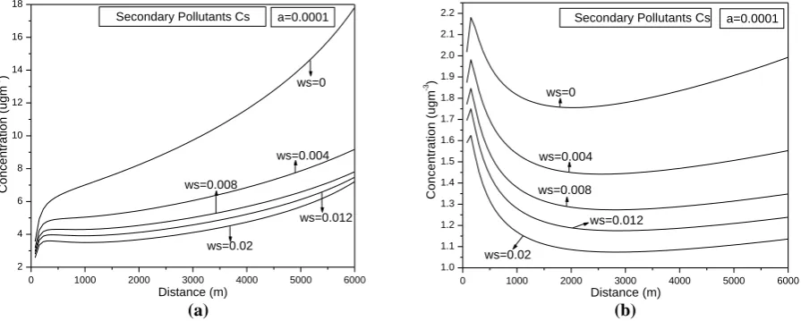
Figure 3: Concentration versus Distance with and without mesoscale wind.

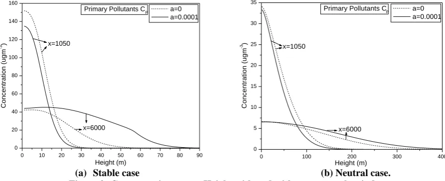
It is evident from the figures 2 and 3 that the mesoscale wind effect on concentration of primary and secondary pollutants is to aggravate the large scale wind. From figure 2 one can observe that at the distance

1050 meters

x the primary pollutants concentration with mesoscale wind is less than that of without mesoscale wind and at the distance x6000meters the concentration is more in the presence of mesoscale wind for both cases. In figure 3 concentration versus distance for secondary pollutants is analysed for both cases of atmospheric stability and mesoscale enhances concentration of pollutants after the center of heat island.

0 5 10 15 20 25 30

(9)

x=1050 Secondary Pollutants Cs a=0.0001

Height (m)

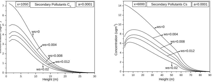
Figure 5: Concentration versus Height for different settling velocities for neutral case.

The examining of secondary pollutants concentration is more essential than that of primary pollutants because of its longer life period and is more hazardous compared to primary pollutants. The variation of secondary pollutants concentration with height at a distance x1050 meters and x6000meters is studied in the figures 4 and 5 for stable and neutral case with mesoscale wind (a0.0001) effect and for different gravitational settling velocities. Here we notice in both stable and neutral atmospheric conditions, the concentration of secondary pollutants reduces as the height increases and becomes zero thereafter. But comparatively neutral condition takes pollutants to a greater heights rather than stable condition. However the concentration of pollutants is more with stable condition compare to neutral. We notice from the graphs that as the gravitational settling velocity rises, the concentration of secondary pollutants reduces for both atmospheric condition of stability.

In figure 6 the plots of secondary pollutants concentration versus distance for different gravitational settling velocities are presented for stable and neutral atmospheric cases. The settling velocity effect on secondary pollutants is uniform throughout the region of study and as gravitational settling velocity rises the pollutants concentration decreases everywhere. Same result is observed for both stable and neutral atmospheric cases but the magnitude of secondary pollutants concentration is high in stable case compared to the neutral case.

0 1000 2000 3000 4000 5000 6000 2

0 1000 2000 3000 4000 5000 6000 1.0

(10)

VI. CONCLUSIONS

A two-dimensional mathematical model to calculate the ambient concentration of air pollutants emitted from a line source in stable and neutral conditions of atmosphere in company with pollutants removal by gravitational settling and the effect of mesoscale type wind and chemical reaction has been presented in this paper. The results have been analyzed in downwind and vertical direction for the dispersion of air pollutants for stable and neutral cases of atmosphere. The mesoscale wind is together with large scale wind reduce the concentration of pollutants to the left of center of heat island and is opposite in direction and hence enhances concentration to the right. We found from the figures that the magnitude of concentration is comparatively more in stable case than in neutral case and the concentration level reaches maximum height comparatively in neutral case than in stable case. This indicates the enhancement of vertical diffusion of pollutants in neutral condition of atmosphere. From the figures we conclude that as gravitational settling velocity rises the concentration of secondary pollutants reduces everywhere in both stable and neutral conditions of atmosphere.

REFERENCES

[1] Yung-Ling Lee & Yueliang Leon Guo, ―Air Pollution and Asthma in Asia‖, Allergy & Clinical Immunology International – Journal of the World Allergy Organization, 16/4, 2004.

[2] Janice J. Kim, Svetlana Smorodinsky, Michael Lipsett, Brett C. Singer, Alfred T. Hodgson, and Bart Ostro, ―Traffic-related Air Pollution near Busy Roads - The East Bay Children’s Respiratory Health Study‖, Am J Respir Crit Care Med, Vol 170. pp 520–526, 2004.

[3] Wolfgang Koch, ―A Solution of the two-dimensional Atmospheric Diffusion equation with

height-dependent diffusion coefficient including ground level absorption‖, Atmospheric Environment, Vol 23. No. 8, pp 1729-1732, 1989.

[4] P. J. Sullivan and H. Yip, ―Near-field Contaminant Dispersion from an elevated Line Source‖, ZAMP Vol. 38, pp 409-423, 1987.

[5] John M. Stockie, ―The Mathematics of Atmospheric Dispersion Modeling‖, SIAM REVIEW, Vol. 53, No. 2,

pp. 349–372, 2011.

[6] Venkatachalappa. M., Sujit kumar khan and Khaleel Ahmed G Kakamari, ―Time dependent mathematical

model of air pollution due to area source with variable wind velocity and eddy diffusivity and chemical reaction.‖, Proc Indian Natn Sci Acad, 69, A, No.6, pp 745-758, 2003.

[7] Krishna S, Lakshminarayanachari K and Pandurangappa C, ―Mathematical Modelling of Air Pollutants

Emitted from a Line Source with Chemical Reaction and Mesoscale Wind‖, International Journal Of Scientific & Engineering Research, Vol 8, Issue 5, pp 48-54, 2017.

[8] Sujit kumar khan, M. Venkatachalappa and N. Rudraiah, ―Time dependent mathematical model for settling

of primary air-polutant and its secondary product‖, Modelling, Measurement and Control, Vol. 61, No. 2, pp 39-55, 2000.

[9] Pandurangappa C, Lakshminarayanachari K and M Venkatachalappa, ―Effect of mesoscale wind on the pollutant emitted from an area source of primary and secondary pollutants with gravitational settling velocity‖, International Journal Of Emerging Technology Advanced Engineering, Vol. 2, Issue 9, pp 325-334, 2012.

[10] Pandurangappa C, ―Mathematical modeling of air pollution problems with chemical reaction and mesoscale

winds‖, Lambert publication 2012.

[11] Jones P M, Larringa M A, Wilson C B, ―The urban wind velocity profile‖, Atmospheric Environment 5, pp

89-102, 1971.

[12] Shir C C, ―A preliminary numerical study of a atmospheric turbulent flows in the idealized planetary

boundary layer‖, J. Atmos. Sci. 30, pp 1327-1341, 1973.

[13] Ku J Y, Rao S T and Rao K S, ―Numerical simulation of air pollution in urban areas: Model development‖,