A Contribution to the Theory of High Frequency Elastic Waves, with Applications to the Shadow Boundary of the Earth's Core

(1)

A CONTRIBUTION TO THE THEORY OF HIGH FREQUENCY Eh~STIC WAVES, WITH APPLICATIONS TO THE

SHADO', BOUNDARY OF THE EARTH'S CORE

Thesis by Paul Granston Richards

In Partial Fulfillment of the Requirements

For the Degree of Doctor of Philosophy

California Institute of Technology Pasadena, California

1970

(2)

i i

ACKNOWLEDGMENTS

The author appreciates the advice given by Prof. C. B. Archambeau throughout the development of this study. Many useful discussions "ere held with past and present staff members of the Seismological Laboratory at the California Institute of Technology, and in

particular with Prof. J. N. Brune (now at the University of California at San Diego).

Prof. T. L. Teng of the University of Southern California worked with the author on a preliminary numerical study of the

solution presented in Chapter 2, section 2, and its geophysical consequences. The author was fortunate in being able to spend four weeks during 1969 at Princeton, where he learned of the recent work done by Prof. R. A. Phinney of Princeton University and

Mr. C. H. Chapman (then visiting from the University of Cambridge) : their contributions to the present study are acknowledged in the text below.

Mr. David P. Hill has given the author valuable assistance, particularly on computational problems.

Mrs. Barbara Sloan typed the" manuscript, and Mr. Laszlo Lenches drafted the figures.

(3)

i i i

ABSTRACT

The diffraction of P and S waves by various obstacles is studied theoretically, in order to evaluate frequency dependent corrections to ray theory for elastic waves which travel nearly along the Earth's core shadow boundary.

Most of the properties of this scattering process are conveniently illustrated by a simple Earth model, which gives rise to a problem in plane strain. This model is an infinite homogeneous elastic solid in which a steady state plane body wave

(of the type P, SV, or SH) is incident on a circular cylindrical cavity. A Poisson summation is used for the scattered elastic potentials, and contributions from waves diffracted at least once around the cylinder are neglected. Simple approximation formulae are developed to examine the behavior of P, SV, and SH waves on and near their geometrical shadow boundary behind the fluid.

Computed numerical results are believed to be valid for frequencies above 0.03 Hz.

The solution method, which may be regarded as a corrected Fresnel theory, is taken through four successive stages of generalization to study increasingly realistic Earth models:

(4)

iv

an ultrasonic model experiment conducted by Teng and Wu (1968). (ii) Diffraction by a fluid cylinder of cylindrical waves from a line source. (iii) Diffraction by a spherical fluid of spherical waves from a point source. Here we find good agreement between numerical results from our approximate method, and computation of the exact Poisson line integral.

The final stage of generalization, to study (iv) diffraction by a spherical fluid/solid discontinuity in a realistic radially heterogeneous Earth, is obtained by methods similar to (iii), but

after an extensive revision of Hook's (1961) discussion of elastic potentials in general media. In our approach, we recognize that

the designation of P and S displacements is somewhat arbitrary in heterogeneous elastic media, but becomes precise in the high frequency limit of ray theory (in which P and two S components

are decoupled). These facts are used for radially heterogeneous isotropic Earth models to establish three potentials (P,S,T)

with the properties (a) that T(r,t) is decoupled from P and S, and ~

is a potential for SH motion, (b) the coupling of P and SV waves is reflected in a system of coupled scalar equations for P(X,t)

and S(r,t), and (c) in the high frequency·.Hmit we have P(r,t)

~ ~

and S(r,t) satisfying canonical uncoupled wave

~

.

1"

(A+21l)t.

IIl

)±

respect~ve ve oc~t~es --p-- \ ; .

equations with

(5)

v

Many possibilities are suggested by the coupled equations for P(~,t) and S(£,t), apart from their use in the solution of

(iv) above. They lead to a statement of conditions on the Earth model under which P and SV waves can propagate independently

(at any frequency). We also use them to obtain approximate

reflection coefficients for upper mantle transition regions which generate observed precursors to the phase PKPPKP, finding that the extent of velocity gradient anomaly in such regions must be less than about 4 km, in order to observe short period (1 sec)

reflections.

Our numerical study of core diffraction provides an

explanation for the observed polarization towards SH of diffracted S waves, and also shows that there is a slight dispersion effect

dT

(6)

vi

TABLE OF COTIENTS

Page

Ch.apter 1

General Introduction--- 1

Chapter 2 Diffracted P, SV, and SH Waves, and Their Shadow Boundary Amplitudes--- 11 2.1 Introduction--- 11

Plan of Theoretical Development--- 14

2.2 Theoretical Development of a Simple Model of Diffraction Statement of Elasticity Problem--- 14

Scattering of p--- 16

Discussion of ~ (i.e. P-P Scattering)--- 18

s Evaluation of $ Near the Upper Shadow Boundary--- 22

s Scattering of SV--- 26

Scattering of SH--- 31

The Shift of Shadow Boundaries--- 32

Numerical Method and Results--- 33

Method--- 33

(7)

vii

Page 2.3 Diffraction of Cylindrical Waves by a Cylindrical

Cavity--- 38

Statement of Elasticity Problem--- 39

Scattering of P-Waves--- 39

Evaluation of al(r,-8)--- 41

Evaluation of a2(r,-8)--- 43

Discussion--- 43

Numerical Results--- 45

2.4 Diffraction by a Fluid Cylinder--- 45

Potentials for PcP and PcS--- 50

Numerical Results--- 54

2.5 Diffraction of Spherical Waves by a Spherical Fluid--- 55

Scattering of SV-Waves--- 60

Scattering of SH-Waves--- 60

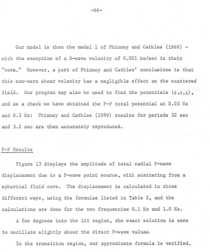
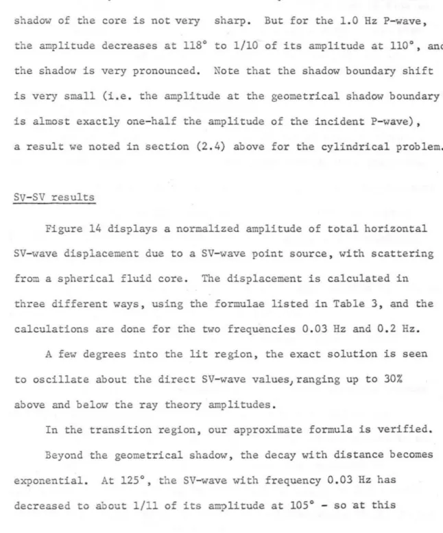
P-P Results--- 66

s

v

-sv

Results--- 67

(8)

viii

Page

Amplitude within the Shadow--- 69

2.6 Body Waves in Radially Heterogeneous Media, Scattered by one Solid/Fluid Interface--- 75

The Expansion of Source Potential, and Potential-Displacement Relation--- 76

Evaluation of the Scattered (PCP) Potential--- 80

Diffracted Arrivals within the Shadow--- 87

2.7 Relevance of our Theory, and Applications to Seismic Data--- 105

P-Wave Amplitudes in the Shadow of the Earth's Core--- 105

S-Wave Polarization--- 107

Theory--- 107

Observation--- 107

Conclusion--- 108

The Phase of Transition Region Body Waves--- 108

Numerical Discussion of Dispersion Effect--- 109

Conclusion--- 119

Chapter 3 Elastic Wave Propagation in Spherically Symmetric Inhomogeneous Media: Potential Methods--- 120

(9)

ix

Page

3.2 A Discussion of the Choice of Dependent Variables--- 124

3.3 Wave Equations for Potentials--- 136

Toroidal Motion--- 136

Spheroidal Motion, Neglecting Self-Gravitation--- 137

3.4 Properties of the Coupled Potential Equations--- 140

(a) High Frequency Decoupling of P and SV Waves--- 140

(b) Comparison "ith Hook's Method--- 144

(c) Brief Summary of Applications and Extensions--- 150

(d) Conclusions--- 163

References--- 164

Appendices--- 175

(1) Formulae for P-S and S-P Scattering--- 175

(a) P-S (See Figure l(b))--- 175

(b) S-P (See Figure 1 (c))--- 177

(2) Expansion of the Point Source in a Smoothly Varying (3) Spherically-Symmetric Medium--- 178

d 2o!> A Proof that d\l2 \I = wp = 1 , "here o!> is the Phase Function of Section (2.6)--- 184

(4) Description of the Program EXACT--- 187

Purpose--- 187

(10)

Page

Choice of Path r-~--- 188

Method--- 189

(5) The

F

resnel

-

Kirch~ff

Method in Radially Heterogeneous

(6)

(7) Media--- 191

Asymptotic Expansion about Turning Points--- 198

dT Inversion of Perturbed d~ Data--- 207

Statement of Inversion Problem--- 207

Solution Method (due to Jeffreys, 1966)--- 207

Application--- 208

(8) Potentials for the General Elastic Solution in Spherically Symmetric Media--- 210

(9) A List of Functions Defined in Section (3.3)--- 219

(10) Some Properties of the Source-Generated Potentials Described in Section (3.4)(a)--- 222

(11) The Reflection and Transmission Coefficients, Between Two Slightly Different Welded Homogeneous Elastic Half-Spaces, for an Incident P-Wave--- 228

List of Tables---~--- 239

Tables--- 241

Figure Captions--- 251

(11)

-1-Chapter 1

General Introduction

Improvements during the 1960's in both the quality and quantity of seismic data have concurrently stimulated considerable interest in an improvement of the theory for elastic waves. The immediate goal of such new theory and data is a more accurate estimation of the longitudinal and shear wave velocities, and density, everywhere within the Earth.

The achievement of this' goal is in turn crucial to that most basic aim of geological science, a full statement of the constitution

and evolution of the Earth, because it appears that from data now available there is a potential for assigning the seismic parameters with great precision. This potential has indeed been realized already throughout most of the Earth, and we may cite for example

the longitudinal velocity distributions of Gutenberg and Jeffreys which had been established by 1939, each distribution differing between depths of 900 and 2800 km by less than 1% from the recent study of Hales, Cleary and Roberts (1968). However, the importance of further data analysis lies in the fact that diagnostic clues to composition are principally contained in regions of high velocity gradient, or of velocity contrast, and such regions are just

(12)

-2-travel time data (see Gerver and Markushevich, 1966, for a

theoretical discussion), and it is necessary to use other

phenomena such as surface wave dispersion (see Brune and Dorman,

1963) or the amplitude of body waves (see Julian and Anderson,

1968) to discriminate further between velocity models.

Ynis study is directed towards improvements of classical

ray theory, and, while several new and quite general results are

p~esented for homogeneous and inhomogeneous elastic media, we

emphasize the particular problems of analyzing core-diffracted body

waves near the shadow boundary.

The geophysical community has seen a large number of publications

reporting theoretical and observed properties of core diffraction

(for a review, see our Introduction to Chapter 2 below), and

there are several reasons why the core-mantle boundary remains

the subject of widespread current research. In summary we

may mention here that theoretical departures from ray methods are

suggested by Johnson (1969) for rays which nearly graze the boundary,

so standard methods for inverting seismic data are suspect. Yet

the determination of present core-mantle boundary parameters is

important both to our knowledge of the present density distribution

throughout the Earth, and to the historical study of core

differentiation. A large amount of relevant seismic data is

available, partly because arrivals in the distance range 85°-115°

(13)

-3

-Alexander and Phinney (1966) have pointed out that comparison

of arrivals in the core shadow which are along the same great

circle path can be used to study lateral heterogeneities at

the bottom of the mantle. A final and basic reason for our examination of the core-mantle boundary is that it appears to be

a simple example within the Earth of a region of varying velocity,

bounded by a velocity discontinuity. This combination is possibly present in several other regions of the Earth (see Archambeau,

Flinn and Lambert, 1969), and also in planetary atmospheres which

have been subjected to occultation experiments, and so our new

theoretical and numerical methods may be expected to find applications

considerably wider than the present study. Our results are

summarized below in this Introduction, but first we briefly survey

the standard wave propagation theories now used in seismology.

Ray theory itself (see Bullen's 1963 text for a summary,

and applications), with its underlying assumption that P, SV,

and SH waves separately obey the laws of geometrical optics, is

an approximation which can provide a basic guide to more exact

methods. This must be true, because the bi-characteristics of the general equations for elastic displacement are identifiable

precisely as rays (see Section (3.2) below). Before developing new

methods, we should thus be aware of two types of problems for which ray theory is essentially exact:

(i) It is exact for problems of plane waves, incident on

(14)

-

4-some e~ceptional problems concerned with grazing and critical

incidence. See Goodier and Bishop, 1952, and Hudson, 1962.)

The case of a curved wavefront can be e~ressed as an integral over plane waves, and the evaluation of such integrals has led

to a vast catalogue of solved problems, for

differentsource-receiver-boundary geometries (for an e~tensive review, see Miklowitz, 1966).

(ii) Robinson (1957) and Vlaar (1968) have shown for

heterogeneous media that a ray theory, based on the concept of

a wavefront as the carrier of a discontinuity in particle velocity,

can give e~act results for the propagating wavefront itself.

Discontinuities in P, SV, and SH are shown to propagate independently

-but behind the wavefront, these displacement fields are, of course,

coupled in ways which ray theory cannot e~ctly interpret.

It is often claimed that ray theory is accurate for a medium

in which the changes in such physical properties as velocity, and

velocity gradient, are small over a wavelength (see Officer, 1958,

and Archambeau, Flinn and Lambert, 1969). While such criteria

can be useful in some particular applications, they must be

in-sufficient in general, since the total path length within the

heterogeneity is not taken into account - if this path length is

sufficiently long, we intuitively e~ect that ray theory must become arbitrarily bad. But note from (ii) above that we also

should e~ect ray theory to be arbitrarily good for a spatially

(15)

-5-the elementary equation for displacement is valid) if the source frequency is sufficiently high. Further breakdown of ray theory occurs in the neighborhood of .caustics (i.e. the envelope of a system of rays), and of the geometrical boundaries of shadows cast by discontinuities within the elastic media.

It is clear then that the approximate solutions of ray theory in seismological applications need checking against exact solutions, wherever this is possible, in order to assess the accuracy of the former method. To this end, we give in Chapter 2 below the exact solution for elastic displacement in simple Earth models, near the shadow boundary due to the core-mantle discontinuity,

and compare it with ray theory and other approximations. In this case we can show by example how the assumption of uncorrected ray theory may consistently bias the conclusions of inversion for mantle velocities just above the core.

Tne device of approximating the Earth by welded layers of homogeneous plates (or concentric homogeneous shells) has led to much successful work. Methods initiated by Thomson (1950), Haskell

(1953, 1960, 1962), and Knopoff (1964) are particularly useful in studies of surface wave dispersion, and of course this type of model is particularly suited to the geophysical problems of inversion.

But there are some strong objections to modelling the Earth by homogeneous plates.

(16)

-6-properties not common in general media. Thus, a calculation of the

travel times in layered models often reveals small triplications

induced by the layering - an inconvenience which usually can be

avoided by using, for example, a Mohorovi~i~ law of inhomogeneity

(i.e. velocity proportional to an irrational power of radius). A

more interesting, but still somewhat spurious, property leads

to the fascinating problem of headwaves; the traveltime for a

head-wave arrival indicates a travel path of critical incidence at one

of the boundaries, together with grazing boundary ray transmission

in the faster medium, and this special property is the basis of

special methods for the evaluation of headwave displacement.

Typically, these are the branch line discussions of, for example,

Berry and "est (1966), or the less ,."ell-known operational methods

of Jeffreys (1926), or studies of wavefront curvature by Yanovskaya

(1968). But even a small velocity gradient destroys the simple

property of critical incidence - grazing transmission; the

theoretical approach to "headwaves" (in so far as this energy

may be isolated) is then either a diffraction study of scattering

poles (if velocity decreases with depth: see Hill, 1970) or a

multi-ray study of saddle points and scattering poles (if the

velocity increases with depth: see

~erve~y

,

1966, Chekin, 1965,

and also Chapman, 1969, for the related problem of SKK ••• KS within

a simple Earth model) . It appears that Runge's Theorem (Hille, 1962)

(17)

-7

-positive and negative gradients (as the gradient becomes smaller),

and the branch line method in the limiting case of two homogeneous media.

The second type of objection is part practical, part aesthetic.

We have considerable evidence (e.g. Johnson, 1967) for regions of

high velocity gradient within the upper mantle, but the number

of homogeneous layers needed to model such a region accurately for

body waves is so large that reflection data (Adams, 1968, and I,~itcomb

and Anderson, 1970) cannot yet be related accurately to the velocity

gradient (although Teng and Tung (1969) have recently reported

some success). And so far as we know, the Earth is not composed

of homogeneous layers, and the coupling between P and SV is not

accomplished by discontinuous boundaries; it is accomplished

intrinsically in the equations of motion.

It seems that the only method which both accepts this last

fact, and calculates its effect, is that initiated by Epstein (1930) ,

which for certain velocity gradients in acoustic media can furnish

an exact solution for the reflection and transmission coefficients.

This method, which transforms the equations of motion into a form

satisfied by hypergeometric functions, and then uses the connection

formulae between different pairs of solutions, is available for a

theoretical study of SH waves. And a conclusion of our Chapter 3

below is that the same method may possibly be used, with an approximate

(18)

-

8-coefficients for the precursors to PKPPKP.

The methods of Phinney and Alexander (1966) and Phinney and

Cathles (1969) have guided several sections of our Chapter 2 below.

Their procedure is to represent the displacement potentials, for

elastic waves in a simple Earth model, in a standard way as complex

line integrals, and to evaluate the integrals numerically. Such

an approach has been slow in finding seismological applications,

since a similar break-through was achieved in 1946, in a study by

Fock of electromagnetic waves - and see also Wait and Conda (1959) .

Recent work of Chapman (1969) has further extended the method in

seismology by incorporating a scheme for direct numerical integration

of the equations of motion through the turning point at the bottom

of a ray path.

The study below is presented in two chapters, which are almost

independent. (Just one conclusion of Chapter 3 is used in Chapter 2.)

In Chapter 2 we solve a simple shadow boundary problem in

elastic plane strain. In several stages we generalize the solution

method to investigate the shadow boundary set up by a point source

in a simple Earth model composed of separately homogeneous mantle

and core. Exact displacements are calculated (by Phinney's method)

for P, SV, and SH sources, and are compared with the approximations

of ray theory in the lit region, and a corrected Fresnel theory

(19)

-9

-We find that the latter approximation (which is found to be quite accurate in the simple Earth models) can successfully be generalized to examine more general Earth models (with radial heterogeneity), giving the combination P + PcP from distances where they begin to interact, out to (and including) the shadow boundary. And a numerical method is given for evaluation of diffracted arrivals in the shadow, back to (and including) the shadow boundary. Both these methods are quite simple to use in realistic Earth models; the corrected Fresnel method is expressed as a factor multiplying the ray approximation for the direct P wave field, and successfully matches the numerical

shadow region method on the shadow boundary. Several implications of our results are described, and include (a) showing that the grazing reflection coefficient for elementary waves at a spherical discontinuity is, for our geophysical parameters, substantially different from the corresponding coefficient with a plane

discontinuity, (b) explanation of the observed polarizing effect, on S waves, of core diffraction, and (c) an evaluation of Johnson's

(1969) caveat, that velocities obtained at the bottom of the mantle, dT

by standard Herglotz-Wiechert inversion of observed d6 values, are too low.

(20)

-10-mathematicians to take advantage of many similarities to be found

bet"een the different problems. The similarities arise because

equations of wave propagation (be they for a magnetic intensity, for

a stress tensor, or for particle scattering) may often be transformed

to and from certain "canonical forms" of wave equation. The widely

studied properties of canonical forms may then be simply related

to our particular problem, provided we can establish the necessary

transformation. Hook (1961) and Singh and Ben-Menahem (1969) have

studied the equation for elastic deformation, but our approach

differs from these authors in using a slightly simpler potential

representation by which (we prove) all possible displacement solutions

can be studied. We are able to see, from our final choice of potentials,

the theoretical reasons why P and SV body waves in the Earth are

observed to propagate almost independently, and the generality of

our final coupling equations permits a survey of many possible

applications. For example, we show the relevance to seismology

of some canonical wave solutions in certain standard kinds of

inhomogeneity, and are able to see that all experimentally

identifiable reflection horizons in the Earth's mantle must be

highly localized.

The new work presented in this dissertation includes our

study of amplitudes near a shadow boundary in homogeneous elastic

(21)

-lOa-heterogeneous Earth models, their eore shadow boundary and shadow

region. The generalizations are examined numerieally for a realistic

Earth model. We also place Hook's method of potentials on a firm and simpler foundation.

(22)

-11-Chapter 2

Diffracted P, SV, and SH Waves, and Their Shadow Boundary Amplitudes

2.1 Introduction

Since the installation of the World-Wide Standardized Seismograph Network, rapid accumulation of seismic data on diffracted body-wave amplitudes has given us hope of better determination of the radius and nature of the Earth's core-mantle boundary. There has been, however, a lack of appropriate diffraction theory for the

interpre-tation of these recorded amplitudes, particularly for observations made near the shadow boundary. This chapter develops a solution for the displacement of body waves which closely graze the core, and the theory is examined in relation to some observed data. It is found that the phenomenon of SH polarization in diffracted S waves, reported by Cleary et al (1968), is qualitatively explained. It is also found that the departure from ray theory in the shadow boundary region may be very simply allowed for when using Herglotz-Wiechert inversion to set up models of the lower mantle (see Johnson (1969): a

dT frequency dependent correction is made to the observed d~ for the interference effect of PcP).

to allow

Displacement solutions that are valid only in limited regions have previously been obtained for some problems with simple

(23)

-12

-elastic solid (Scholte, 1956; Duwalo and Jacobs, 1969; Knopoff and Gilbert, 1961), and scattering from a rigid cylinder or sphere (Gilbert and Knopoff, 1959). Some of these solutions are for impulsive elastic waves, and so are unsuited to the interpretation of spectra. All of these solutions are valid only within the

"illuminated" region (that is, the region accessible to direct body waves from the source), or within the shadow boundary, and they

fail for regions near the geometrical shadow boundary. The failure of these theories in the critical region of core- grazing rays has hindered meaningful discussion of the observed diffraction data - for presumably it is just these rays which provide the best information we have on core-mantle structure.

Recent progress in acoustics and electromagnetics has provided solutions valid in the neighborhood of the geometrical shadow boundary, for scatterers of various simple geometrical shapes (Rice, 1954;

Rubinow and Wu, 1956; Rubinow and Keller, 1951; Nussenzveig, 1965). Although these results are not immediately applicable to the study of elastic waves, the gross structure of the solutions and the general conclusions are expected to be common to all wave-scattering problems: typically, their findings are

(1) a broadening of the transition zone (that is, the region between illumination and shadow) with lower frequency, (2) a dependence of the extent and position of the transition

(24)

-13

-(3) strong similarity among solutions for spherical, cylindrical,

and paraboloidal scatterers with the same boundary condition.

The theory of this chapter is an extension to seismology of the

solution techniques developed in acoustics and electromagnetics, and

we examine the amplitude behavior of P and S-waves near the geometrical

shadow boundary. This extension involves the study of more general

boundary conditions that couple two potentials and their derivatives,

as opposed to the Dirichlet or Neumann conditions considered in

acoustic and electromagnetic problems. A substantial extension to

the theory of radially heterogenous media is also given.

We are fortunate in having two independent checks on the theory

of this chapter. An ultrasonic seismic model experiment (Teng and

Wu, 1968) has been conducted, which measured transition amplitudes

of P and SV behind a circular hole cut in a thin plate. Also, a

method of Phinney and Alexander (1966), and further described in

Phinney and Cathles (1969), has given transition amplitudes of a

P-wave potential due to a fluid spherical core. The method of

Phinney and his co-\"orkers, which involves extensive numerical

integration, is described belOt". The results of both the above

(25)

-14

-Plan of Theoretical Develoument

The simplest geophysically relevant problem of elastic wave

diffraction is a problem in plane strain: a steady state plane wave

of displacement is incident upon a circular cylindrical cavity, and

it is required to evaluate displacements near the geometrical shadow

boundary. This basic problem is solved in section (2.2). The

generalization to diffraction of waves from a line source, and a

comparison of theory with the results of Teng and Wu (1968), is given

in (2.3). In (2.4), we generalize to the case of a fluid cylindrical

scatterer, and in (2.5) we solve the parallel problem of a point

source, with waves scattered by a' spherical fluid, and compare the

results of Phinney and Cathles (1969). The generalization to a

radially heterogeneous Earth is made in section (2.6). In (2.7) we

apply our new results to observed phenomena.

2.2 Theoretical Develoument of a Simple Model of Diffraction

Statement of Elasticity Problem

A steady-state plane wave of unit displacement is incident from

the left on a circular cylindrical cavity of radius a (see Figure l(a)).

This is a problem of plane strain, and we wish to evaluate the scattered

(26)

-15

-We use polar coordinates (r,6,z) centered on the cylinder axis,

and shall consider the cases of

1. Diffraction of P-waves with a plane P-wave incidence:

i(hr cos6 - wt) u. = (cos6,-sin6,0) e

"'.I.

2. Diffraction of SV-waves with a plane SV-wave incidence:

_ ( . 6 6 0) i(kr cos6 - wt)

u. - sln, cos, e "'.I.

3. Diffraction of SH-waves "ith a plane SH-wave incidence:

u. = (0,0,1) "'.I.

i (krcos6-wt) e

For the P-wave due to SV-wave incidence, and the SV-wave due to P-wave

incidence, formulae are given in Appendix I.

In the first two cases, our problem can be reduced to a !';o

-dimensional one involving !';O scalar potentials

q.

and 'iJ , which are

related to the displacement field u by ~

(2.2.1)

The total displacement ~ is a solution under the conditions

(i) that (V2

+

h2)q.

=

(V2

+

k2)'iJ

=

0, where (h,k) are the wave

(27)

(ii)

-16-that the scattered waves u _ u - u. are outgoing, and

"""

~

'"""-(iii) that there is neither tangential nor normal stress on

the boundary r

=

a.

Scattering of P

The incident wave clearly may be represented by

i(hrcos8-wt) d ,"

e ,an 't'. =O.

~

The conditions (i) and (ii) allow us to write scattered potentials as

1

ih

lVe can evaluate

relation

A n

e

and B by

n

i hrcos8 =

H(l) (kr) n

using condition (iii) ,

00

L

(i)n J (hr) e in8 n

n=-co

i(n8-wt) e

(2.2.2) .

(28)

-

17-This procedure is straightforward, but lengthy, and gives

1

°1

H(2) (ha)

=-

t[::

J (ha)

J

1

+

n B n (2.2.3)

A

-Z

H(l) (ha) H(l) (ha)

n

°1

n n n

where for convenience we have defined operators

°

H (R.) (ha)

1 n

=

S(l)p(R.)

+

Q(l)R(R.) R. = 1,2

02J (ha) _- i [R(2)p(1) _ R(1)p(2)] n

where

p (.I.) _2ha_Hn₍_R._)'_(ha)

+

[

_{k2a 2}_- _{2n2] H}₍_R.₎_(ha) (2.2.4)

- _n

Q (R.)

- -2n (ka

H~

R.

)

'(ka)

_H~

R.

)

(ka) )

R (R.)

- 2n ( ha

H~

R.

)'

(ha) -

H~R.)

(ha»)

S (R.)

- 2ka H (R.) , (ka)

+

k 2a 2 - 2n2 ] H (R.) (ka) •

n n

Each of the A and B may now be evaluated, for specific values

n n

of w,a,~ and S: the unique solution for u follows from equations ...."

(29)

-18

-Discussion of

¢

(i.e. P-P Scattering) s

It is unfortunate that the series solutions (2.2.2) converge

so slowly that they are of little direct use. It is clear from

the form of (2.2.3) and (2.2.4) that, if there is convergence, it

must be slow, for A is small in general only for n »ha. For a n

simple model of the Earth's core-mantle boundary, we find for body

waves with period 1 to 50 seconds that ha varies between 1600 and

30 (and ka between 3000 and 60).

However, if we wish to find $ for values of (r,B) in the

s

illuminated zone, and for an incident wave of frequency high enough

for us to expect a reflection effect, we can make an estimate of the values of n which we expect physically to be most significant.

These values are integers which most nearly satisfy the relation (see Figure 2)

n w r sin i(r)

a (2.2.5)

(The corresponding relation for a spherically symmetric body is

+

1

___

w r sin i

n ; see Bremmer (1949), Ben-Menahem (1964).)

2 a

(ina-wt)

A simple way to obtain (2.2.5) is to use the factor e

in the n-th term of the series (2.2.2). This factor indicates that each term of the series represents a wave travelling around the

cavity with phase velocity v =

n n

wr

(30)

-19

-The summation ~ represents an interference effect of all these s

different phase velocities, and the reflected-ray phase velocity is (see Figure 2) - a/sin i in the direction of increasing e.

The interference is thus constructive only "hen v =-~ wr - 0 ,i.e. n n sin i

when (2.2.5) is nearly satisfied. For (r,e) near the shadow boundary, we have r sin i ~ a, so the significant terms are n ~ - ha. The quantity r sin i

a in (2.2.5) is the familiar seismic ray parameter, and part of the above theory has a generalization to radially heterogeneous models (see section

(2.6»

.

We now proceed to an evaluation of $ for large values of ha, s

using the Poisson sum formula. Our development has been guided substantially by the methods of Rubinm, and Keller (1961), who discuss a problem with only one potential and with a different boundary condition on r = a.

A

factor exp(-iwt) is understood in some of the expressions below.

If we define

A(r,e) H(l)(hr) d\l

\I

and use the Poisson sum formula (Morse and Feshbach, 1953)

(31)

with

1 F(n) =

ih

we see that

cPs

in1T/2 e

1

-

_2ih

-

-20-A H (1) (hr) n n

in6 e

A(r,2m1T

+

6) (2.2.6) •

In this exact formula for cP we wish to identify waves that travel s

around the cylinder and are then summed to give the scattered field. For example, we note that, for large ha and m ~ 1, A(r,2m1T + 6) has a phase ha(2m1T + 6) and hence represents a wave that has

travelled m times around in the direction of increasing 6. To make further identification it is helpful to rearrange the terms in

equation (2.2.6), to reveal also (1) which waves travel around in the direction of decreasing

e

,

(2) which wave just grazes the cavity for a field point near the upper shadow boundary, and (3) which wave is diffracted around the lower part of the cavity. We are

guided towards the correct rearrangement by noting that physically we expect <p (r,6) = <p (r,-6) and in particular that the upper

s s

(32)

-21-Using

the relations

and

(2.2.6)

becomes

( A(r ,2m" +6) + A(r ,2m"

-

e

))

1

j

+{

f.i

"

I'll

Hv

(1)

(h

r

)dv

+

J~

e

i

(e-1)

n

H (2) (ha)

H (1) (h r) _1 --;V,,=", _ _

v

n

H(l) (ha)

1 v

o

H(l)(hr)dv

'

v

'

+

J

~

i

V

'

(-e~2)

e

H(l) (hr)

v

'

_

nl

_

H..:;,~7,,)

_

(h

_

a

_

)

dV

}

]

n

H(

l) (ha)

1

v

'

(33)

-22-Evaluation of ~ _s Near the Upper Shadow Boundary _.

The first infinite sum in (2.2.7) represents waves that, from

their phase, we identify as having travelled m times (m ~ 1)

completely around the cylinder. These waves attenuate with distance

1

at a rate proportional to (ha)' and arrive much 1ate~ outside the

time-window we are interested in, so we may ignore them. The integrals

in the remaining two brackets { }'represent waves which have not

travelled completely around the cylinder.

From the interference argument mentioned above, we expect to

get contributions for the integrals in (2.2.7) from those regions near v'

=

-

ha and (since in fact v'

=

-

v) v' ha. Near

the upper boundary of the shadow, the second bracket { } is then seen to be negligible relative to the third. Just the opposite

is true when we consider the lower boundary of the shadow (but

with contributions still coming from ·v

=

-

ha, v'

=

+ ha) . Our

interpretation is thus that the second bracket describes the wave

travelling via the bottom of the cylinder, and the third bracket

that via the top. For our evaluation, the diffracted contribution

via the bottom of the· cylinder is negligible, and we may take just

(34)

-

23-1 ~\I

-

e

-i-f

H~

) (hr)d\l +

f

e

~.( 1T)

,

for (ha)3 » 1 ,near t h e upper s h d a ow oun b d ary.

Following Rubinow and Keller (1961), we use

where

al(r,-e)

f

ha i\l (-e+1T/2) (1)

_ e H (hr)d\l

\I

o

ha

I

i\l(-e+1r/2)

a2 (r ,- 6) " e

n

H (2) (ha)

_1 ...:;\1-=-<"" _ _ H (1) (hr) d\l

n

H (1) (ha) \I

1 \I

+

r

ei\l (-6+,,/2) [

ha

To evaluate aI, we may use the Debye formula for H(l) (hr)

\I

(35)

-

24-(2.2.8) .

This integrand has just one stationary phase point, given by a value

v

=

v

such that s

e

Le. v

s hy.

For P(r,e) near the upper shadow boundary (see Figure 1), this

stationary phase point is near the upper limit of integration in

(2.2.8). Making the definition

(v-v)

s

and expanding the phase within (2.2.8) as powers of ~, we find

ihx 2 - i7f /4

al(r,-8) ~ e ' e •

.;;

j

(~j

(a-y)

-

(~jy

i~2

e d~ • .

The upper limit is small near the shadow boundary, and the lower

limit is large for high frequencies; so this Fresnel integral may

(36)

ihx al (r,-6) - e

1

Oxf

y » 1

-25

-i f both

and

(~J!;.

I

a-y

I

« 1

For regions in which the second condition is invalid, al(r,-6) may

be found from a table of Fresnel integrals.

To evaluate a2(r,-6) , we may still use the Debye expressions

for H(l) (hr) and find near v = ha that

v '

i (hx

-- e

11/4)

.

(

_

2

)3:

1Ihx

But, for

H(~)

'

(ha) and

H(~)(ha) (~=

1,2), the simple Debye

v v

approximations are useless. Since argument and order are nearly

equal, some form of Langer approximation is necessary (see "Higher

Transcendental Functions" by staff of the Bateman Manuscript Project,

1953, Vol. II, p. 89), and we discuss this below in the section

(37)

-26

-Then

a2(r,-9)

and Cp(w) is evaluated below, numerically.

In summary: we have for 4> = 4>. + 4> that

~ _s

~

ei(hx-wt)

{1:.

_

(

_

1

)

i

¢

ih 2 2r.hx

-iTT

/4

[

e h(a-y)

+

Scattering of SV

The incident wave may be represented by

.!..

(ha)3

1 i (krcos 9-wt)

ljJi ik e

The conditions (i) and ("ii) allow us to write

i(n9-wt) (i)n C H(l) (hr) e

n n

where

(2.2.9)

(2.2.10).

(2.2.11)

00

1 ~ (i)n D H(l) (kr) e i (n9-wt)

- ik L n n

(38)

-27

-and condition (iii) then gives

1

n4

J (ka) ]

[

n3

H(2) (ka) ]

C =

-

"2

H~l)

(ka) ) D

=

1 1

+

n

n3

n

-

"2

n3

H~l)

(ka)

where we have defined the operators

, R, 1,2

d P (R,) Q (R,) R(R,)

s

(R,) d f· d <n

an , , , are e 1ne •

Discussion of ~ (i.e. SV-SV scattering)

s

(2.2.4) .

(2.2.12)

(2.2.13)

We use a Poisson sum formula, just as before. Thus, defining

V(r,S)

-

r

e

iV₍_S₊_1T/2)

H(l)(kr) dv

(39)

-28

-we have

00

ljis

=

+

2~k

L

V(r,2m1T+e).

m--We find that this sum may be rewritten and interpreted term by term just as we interpreted equation (2.2.7), so that for an evaluation near the upper boundary of the shadow we have

1

{

f

oo

iv(-e+n/2) (1)

lji s = + 2ik e Hv (kr) dv

o

-/

n

H (2) (ka)

3 v

H (1) (kr)

v

(40)

where

d2 (r

,-

e)

-

29-_

f

ka

iV(-e+1T/2) (1)

e H (kr) dv

Q

=_

f

ka e iV(-e+1T/2)

+

r

eiV (-e+1T/2) [

ka

v

dl corresponds to al above, and so

i f both and

(~x)~

I

a-y

I

« l.

H(l) (kr) dv . v

To evaluate d2 near the upper boundary, we may again use the

(41)

-30

-I

e i\l(-6+;r/2) H(l) (kr)- e i (kx-;r/4) ( 2)"i near \I

=

ka.

\I '\ ;rkx

For H (2) '(ka) and H (2) (ka) (2 1,2), we shall use the Langer

\I Ii

approximation. Then

where

.L d2(r,- 6) _ ( _2_

)2-lIkx

C SV(w) = _1_ , [ (ka)l

i(kx-1I/4)

e •

J.

(ka) ,

d\l +

r

ka

The function CSV(w) is evaluated below, numerically.

that In summary: we have for $

=

$. + $

~ s

(2.2.14)

i(kx-wt) e

-ik

1 1 >. -i 11 / 4 . "3

{

.I. [

'J}

Z - ( 211kX) e k(a-Y)+(ka) CSV(w)

(42)

-

31-Scattering of SH

. i (krcos e-wt)

The incident wave has its d~splacement u.

=

(0,0,1) e

"'l.

parallel to the axis of the cylinder. The z component of the

dis-placement satisfies the scalar Helmholtz equation

(,,2

+ =

a

and the stress-free boundary condition on the cylindrical boundary

r = a,

11

a

u =

a

ar z

This boundary condition has been studied by Rubinow and Keller (1961) , and from their results we have

,., (0,0, 1

2 e

-irr

/4 [ k(a-y)

where

- 0.4321 x (1

+

f3

i)

(43)

-32

-This asymptotic solution is valid for

y » 1

The Shift of Shado" Boundaries

Using Cartesian coordinates, "e see from equations (2.2.1) and (2.2.10) that the total P-"ave displacement field near the upper shado" boundary for P-P scattering is

e -irr/4.

- - y.

( 2rrhX) ..

-3irr /4

e _, _{0) ei(hx}_-_w_t)

' (

_2rrhx

)V

;.

From this expression, "e see that on the geometrical boundary y = a

u +

(i,o,o)

_ei(hx-wt) ₌

2

1

%.

as w-+ oo

Therefore, follo"ing the method of several other authors [for example,

Rubino" and Keller (1961), Nussenzveig (1965)], "e make the practical

definition that the shado" boundary for finite frequencies is the

(44)

-33-\V

l

if (ha) » 1, the shadow boundary is y ~ a + sP' where sp is the

"shadow boundary shift," and

(2.2.17)

Similarly, for SV-SV scattering, we have

(

irr/4 1 -iTf/4 [ "

e e ''3

.::

-

( ):l:':2

-

:i

k(a-y) + (ka) 2Tfkx ( 2rrkX)

and (2.2.18)

For SH-SH scattering u is given by equation (2.2.16)

and sSH

~

-1.1806 (karJ a- (2.2.19)

Numerical Method and Results

Method

He present here the evaluation of C

E (w) and CSV(w) (see

equations (2.2.9) and (2.2.14)), and of amplitudes near the shadow

boundary.

(45)

-

34-a of 13.6 km/sec, and an S-wave velocity

e

of 7.5 km/sec, and

embedded in it a cylindrical cavity of radius a = 3480 km. These

assumptions make the computational results also comparable to

previously obtained model-experiment data (Teng and Wu, 1968).

, I

Although the theory is valid for (ha)3 » 1, (ka)3 »1, the computation

was made over the frequency range 0.01 Hz ~

f

~ 5 Hz, which corresponds

to intervals 16 < ha < 8000, and 30 < ka < 15000. A general Hankel

subroutine described by Berry (1964) was modified and incorporated

into the program.

Inspection of the integrands for Cp(w) and CSV(w) shows that

three types of numerical evaluation of Hankel functions are

required.

(i) For Cp(w) we need

H~l)(ka)

and

H~l)'

(ka) for v near ha.

These two functions are oscillatory.

(ii) For CSV(W) we need

H~l)(ha)

and

H~l)

'

(ha) for v near ka.

These two functions are exponentially large.

(iii) For both Cp(w) and CSV(w) we need

H~k)(z)

,

H~k)'

(z)

(k=l,2) for order v varying in value near fixed z.

(z = ha or ka.)

In fact, in cases (i) and (ii) it is only the ratio H(l)' (z)/H(l)(z)

v v

R(v,z) (say) which is needed, with v not near z. R satisfies exactly

(46)

-

35-R' = -

~

- ( 1

-

~)

- R2, and R varies slowly. So

approximately

R(v, ka) _- _2ka1

+

_i_[ ₁

-

k2ii2

v2 - 1 ]

±

for v near ha

4k2a2

1

R(v, hal

_

-..1

_

_[ _-₁ v2 1

J

~

for v near ka.

2ha

+

h 2a 2

+

4h2a 2

Calculation of R by these formulae is correct to within 1%, when

checked against values returned by the HANKEL package. So this

approximation is used in cases (i) and (ii).

For cases (iii), the HAhTKEL package uses Langer approximation

in the form

, k 1,2,

where ~ = v (tanh n - n) and n = cosh-1

viz

.

A subroutine for Hankel

functions of order 1/3 is included, and H(k) ' (z) is found from the

v

recurrence relation H(k)' (z)

=

H(k)(z) -

(viz)

H(k)(z).

v v v

The numerical evaluation of case (iii) was checked against

(47)

f

z H~2) (z)

H(l) (z)

v

_ 00

-

36-C

2 " lZ 3l

[

f

Z _H V7:( 2,,) " (_z_)

H(l) • (z)

v

dv

+

H(2)' (z) + v

H(l) • (z)

v

}]

(2.2.20)

-

z

Rubino" and Wu (1956) sho" that i t is only the region of Langer approximation "hich contributes to the integral, and after path

deformation and residue summation obtain

Cj'" 0.49808 x (1

+

/3

i) C2 '" -0.4321 (1

+

/3

i) . (2.2.21)

Using our HANKEL package, together with a Simpson integration method,

"e find Cj and C2 are indeed almost independent of z, for the range

16 < z < 10,000, since Rubinow and I'u's values are returned to within

1 %

"2

00

The integration path for Cp(w) and CSV(w) in equations (2.2.9)

and (2.2.14) is the real order axis. Although this is an adequate

path for numerical evaluation, a better path is that shown in Figure 3.

Whenever a complex path might involve extra contributions, from

complex poles not near A, the real axis integration was evaluated

(48)

-

37-integrand decays exponentially on either side of the point A, where

, ,

- 3

order equals argument, and a path length of about 4z' or 5z is all

that contributes. For a real axis integration, the integrand to the

left of A oscillates with slowly decreasing contributions as the

,

frequency of oscillation increases, and a path length of about 15z'

,

or 20z must be taken.

Results

We first present in Figure 4 the computed complex functions

Cp(W) and CSV(w), for the frequency range 0.01 Hz - 5 Hz. The

computation becomes less relevant near the low-frequency end - because ,

then (ha)'

~

2. Nevertheless, some values are presented for these

low frequencies, and the theory is believed to be good for frequencies

above 0.03 Hz.

It is interesting to compare the results for elastic waves with

the results for acoustic waves. Figure 5 shows the quantity

H

=

IRe C + 1m C], which is proportional to the shift s of shadow boundaries. H is a negative constant for a hard cylinder ( on which

the normal derivative of the field vanishes) and is a positive

constant for a soft cylinder (on which the field itself vanishes)

(see Rice (1964); Rubinow and Keller (1961). In fact, for a soft

cylinder H = Re C

l + 1m Cl (see equation (2.2.21)) , and for a hard

cylinder H

=

Re C

2 + 1m C2)). Thus we see that for our SH-wave

(49)

-38-incidence, H becomes frequency dependent, tending with high

frequencies to the acoustic soft cylinder value - a fact we can

expect by seeing directly from (2.2.9) and (2.2.14) that C

(w)

and

P

CSv(w) both tend to the integral for Cl (see (2.2.20)) as w +

=

.

The shifts of the shadow boundary are shown in Figure 6. At a

given frequency, incident P- and SV- waves would "feel" an effectively

1argor scatterer than its true size, whereas SH waves would "feel" a

smaller one. At high frequencies, all shifts correctly approach

zero (i.e. the shadow boundary approaches its geometrical limit) .

At lower frequencies, the amounts of shadow shift for different

wave types diverge. For long period body waves, e.g. with period

20 seconds, the cylindrical scatterer of radius a

=

3480 km would

seem to be 90 km (2.6%) larger to P-waves, and 290 km (8.3%) larger

to SV-waves, but 150 km (4.3%) smaller to SH-waves.

Further discussion of these results is deferred to the following

sections, in which we develop (1) the generalization to a line source,

and can thus compare our theory with the results of Teng and Wu (1968) ,

and (2) the generalization to point source and spherical scatterer,

permitting comparison with Phinney and Cath1es (1969).

2.3 Diffraction of Cylindrical Waves by a Cylindrical Cavity

The nature of the diffraction of a cylindrical wave by a cylinder

(50)

-

39-diffraction of a pl~,e wave (see Shenderov (1962)) . This is because

the amplitudes of incident and scattered waves decay with distance

according to the same law, for cylindrical incidence, but a plane

wave does not decay at all. However, we shall see below that for the

intermediate distances of geophysical interest, the field set up by

cylindrical incidence can be quantitatively derived in a very simple

way from the plane wave cases considered in Section 2.2.

A steady-state cylindrical wave of displacement, emanating

from a line source at distance b from a circular cylindrical cavity

of radius a (see Figure

7),

is incident from the left on the cavity.

I,e wish to evaluate displacements near the shadow boundary.

Scattering of P-Waves

In order to obtain the simple form

ihR

e

for the incident

displacement (at high frequencies), we choose the displacement

potentials

-iwt

(51)

-40

-An application of Graf's addition theorem (Watson, 1958) gives

n=-CXI

So we take

H(l) (hb)

n

~ _s

inn/2

e

inn/2 i(ne-wt)(f b)

e • e or r < •

A H (1) (hr)

n n

B H(l) (kr)

n n

inn /2 i(n9-wt)

e e

(2.3.1)

The boundary conditions of zero normal and tangential stress on r

=

a then give the forms (2.2.3) for A and B , i .e.

n n

A

=

n

1

2

where 01 and 02 are defined in (2.2.4) .

Hence we see that the step by step methods of section (2.2)

may be duplicated for the problem of a line source. After identification and rejection of waves which travel around the cavity, and the

(52)

-41-where now

o

EvaluAtion of aj(r,-S)

ivrr/2

e

n

H (2) (ha)

j v

H(l) (hr)dv v

H(l) (hr)dv.

v

Since hr, hb are bigger than v throughout the integration, we

may use Debye expansions to see

aj(r,-S) - - e 2 -2irr/4

rr

o

(53)

-42-This integrand has just one stationary phase point, given by a value such that

a

i.e. v ; hy (see Figure 7).

s

For P(r,a) near the upper shadow boundary, this stationary phase point is near the upper limit of integration. Making the definition

we find

al (r ,-8) ~ e ihR

(v-v ) and expanding the phase in powers of ~,

s

2 -2in/4

- e

n

r ' J

Ir~R

I ei (hR-n/4) [ 1 + e-in/4

J;~~R21

(a-y) ] i f both

(54)

-

43

-Evaluation of _{a 2 (r,}-9)

I.]e may still use the Debye expressions for H(l) (hr) , H(l) (hb)

v v '

and so near v = ha

2 e -i1l/4 e i(hR-1I/4)

11

2 e-iTr /4

~

-"h

~/;::;R;1:;R=2

i(hR-1I /4)

e . Then

where Cp(w) is the function defined above for plane incidence, in

equation (2.2.9).

In summary: we have for <I> =

Discussion

4>. + <I> that

]. s

t

+

(ha)

(2.3.2) •

We see from (2.3.2) that in the neighborhood of the geometrical

shadow boundary (which is given by y = a) the P-wave displacement due to a line source is still directed along a ray from the source,

(55)

ihR

e -irr/4

e

He still have the result

1

-44

-~ +

2

~on the geometrical shadow boundary, as w +~,

(2.3.3)

so we may still define the shadow boundary shift as the distance from geometrical shadow boundary "to the half amplitude line. From (2.3.3) we see that the half amplitude line still has the equation y

=

a + s ,

p

where sp is the shift for plane waves (see 2.2.17) . But this line is radial to the source, and hence diverges from the geometrical shadow boundary. In fact, we see

R

SHIFT

I

P-wave, line source

= - x SHIFT

I

Rl _P-wave_, _{plane source}

~l

x [Reep (w)

+

ImS> (w) ]

-'1

(ha) . a

(2.3.4) The simple geometrical relation between the shifts for a line source and a plane source is illustrated in Figure 8.

(56)

-45

-Numerical Results

A model experiment described by Teng and Wu (1968) gives several

measurements of the shadow boundary shift for P- and SV-waves. Their

Model I and Model II, illustrated in Figure 9, were thin sheets of aluminum with a "pulse" of one dominant frequency, and with a circular hole as the scatterer. The velocity of P-waves in such a plate is

given by

a = (for Lame cons tan ts A and ~, and density p) ,

since we can assume this is a system in plane stress (see Love, 1944, p. 208). Table 1 shows the shifts calculated from our theory

(equation (2.3.4)), and Teng and Wu's experimental values. Also in this table is the geophysical body-wave period for which the model is scaled.

The methods of this chapter receive encouraging confirmation from the agreement in Table 1 between theory and experiment. But direct application of our theory to diffracted seismic waves still requires additional generalization, given in the following sections.

2.4 Diffraction by a Fluid CYlinder

(57)

-46

-The boundary conditions become much more complex, and we must allow

for internally reflected waves. But solution of this problem is

important in geophysics, since we have seen that we expect the location

of the shadow boundary to be dependent on physical properties at the

core-mantle interface. We shall see below that our theory requires

very little extension to accommodate the case of fluid scatterers.

A steady-state cylindrical wave of displacement, emanating from

a line source at distance b from a circular cylindrical fluid of

radius a (see Figure 7) is incident from the left on the fluid. We

wish to evaluate displacements near the shadow boundary. We take

p, h, k as the density, and P and SV wave numbers in the solid,

and p', h' as density and wave number in the fluid.

Scattering of P-waves

As in section (2.3) , we take

~.

=

;rr-;

e-iTI/ 4H(1) (hR) e-iwt

1 /~ 0

$. = O. Clearly, we may solve for the total scattered field by

1

(58)

-47-~

H(l)(hr) i(ne-wt)

T

L

P-wave r > a

~ ~ a

.

e

s n n

n=-~

,T _{b H(l) (kr)} _SV_-_wave _{in r} _>

~s _n _n

'T

~s a' J (h'~ P-wave in r <

n n

(2.4.1)

and then solving for (a , b , a') from the continuity of radial

n n n

displacement, and tangential and normal stress, across r a. But a

a

for a source emitting waves with high frequency energy, it is standard seismological practice to separate a record into P, PP, PcP, PKKP, etc., and to think of these phases as having different ray paths. The

potential

~

!

of (2.4.1) includes all such contributions (except the types PP, PcPPKP, etc. , which involve reflection from the free surface), and the problem of splitting

~

T

for these phases is quite

s

(59)

-48-This is done by showing that the solution for each a , _n b in (2.4.1)

n

can be written as a geometric progression in the form

H (2) (ha)

{,eel

+

(H(l) (h'a)

r

1

w

1 1 n _(LL

I).

L

(L'L,)N n ·(L'L)

a = +

-H(l) (ha)

n 2 2

N=O H(2) (h'a)

n n

b =

t

(1) (LT)+(LL')·

L

H(2) (ha) { w

n . H (ka) N=O

n

(L'L,)N (_Hn7,(l,..,.)_(h_'_a_)

)N+l

.

(L'T}

H(2)(hla)

n

where the symbols (LL), (LL'), (L'L'), (L'L), (LT) , (L'T) (of Scholte,

1956) may be identified as reflection and transmission coefficients

in the following way: the term with index N represents (when

slli~ed over n in (2.4.1)) an arrival which approximately has the

phase appropriate to a ray path made up by

N

internal reflections

within the core. That is, PKK •• ·.KP (for an)' and PKK ••• KS (for b n),

with N

+

1 K1

s in each case. The initial terms,

1

2

H (2) (ha)

n

H(l) (ha) n

H (2) (ha)

(LL) ] =:

n

--'H ("-1-0-) -(h-a-) (LT) - B n n

A n

(say)

(60)

-49

-represent arrivals with the respective phases of PcP and PcS,

so these are the terms which we wish to study. (Note that since

we have a steady state source, the signals coming along all the

different possible paths are superimposed. So the identification

of specified modes of 'propagation is performed by studying their

phase, and not their travel time) .

The manipulative procedure for obtaining the above expansions

of (a , b ) is quite lengthy, and so an alternative method is n n

given below for the introduction and calculation of the required

(A , B). It may be shown that the same result is reached by

n n

(61)

-50-Potentials for PcP and PcS

The n-th partial "ave component within the fluid is chosen in equation (2.4.1) to have the factor J (h'r). This choice must be

n

made to avoid any singularity at r = O. But J (h'r) is a sum of

n

ingoing and outgoing waves, although the system of a P-wave source and conversion to PcP, PcS requires only an ingoing wave within the

fluid. (Tne outgoing wave within the fluid may then be thought of as generated by reflection in the origin: upon reaching r = a, it

generates PKP, PKS, and another ingoing component in the fluid.) Hence, for our examination of PcP, it is necessary to ignore

H(l)(h'r) terms within the fluid, and we use potentials (cf equation

n

(2.3.1»

1jJ

s

o

-iw/4

/Th"

e H(l) (hb) _n

n~-c:o

inw/2

e A H (1) (hr)

n n

B H(l) (kr)

n n

A'H(2) (h'r)

n n

inw /2 i(nS-wt) e e

(62)

where

-51

-The boundary conditions on r = a then give

1

B = -

-n 2 _Q _{H (1) (ha)}

5 n

Q H(~)(ha)

5 n

p' (2)

u.

(2)

_ . ( (2) [ (l) P' (2) (l)J (1) [ ( 2 ) P' (2)u(2)])

Q6J (ha) =

+

1. R P - (2) U - R P - (2) •

n U. U'

(63)

-52-Since the operator Os obeys the same reflection rules as OJ ,

(1) 21fiv (1)

namely 0sH (ha) = e 0SH (ha),

-v v

the methods of section (2.3) for scattering by a cavity may now be

applied for the present problem of scattering by a fluid. We find

the asymptotic solution for P-wave displacement is still directed

along the ray from the source (see Figure 10), and is given by

ihR e

e -in /4

and the shadow boundary shift is

SHIFT,

P-'tV'ave, line-source,

fluid scatterer

where

[

I/~

FLUID

l}

h(a-y) + (ha)

cP

(W)J'

(64)

-53

-Theoretical consideration of an SV source leads to a result just

like (2.4.4) , but with C!LUID(w) replaced by