DOI : https://doi.org/10.32628/CSEIT1952277
Breast Cancer Prediction using SVM with PCA Feature Selection Method
Akshya Yadav1, Imlikumla Jamir1, Raj Rajeshwari Jain1, Mayank Sohani2
1Computer Engineering Department, MPSTME, NMIMS, Shirpur, District: Dhule, Maharashtra, India
2Assistant Professor, Computer Engineering Department, MPSTME, NMIMS, Shirpur, Dis-trict: Dhule,
Maharashtra, India ABSTRACT
Cancer has been characterized as one of the leading diseases that cause death in humans. Breast cancer, being a subtype of cancer, causes death in one out of every eight women worldwide. The solution to counter this is by conducting early and accurate diagnosis for faster treatment. To achieve such accuracy in a short span of time proves difficult with existing techniques. Also, the medical tests conducted in hospitals for detecting cancer is expensive and is difficult for any common man to afford. To counter these problems, in this paper, we use the concept of applying Support Vector machine a Machine Learning algorithm to predict whether a person is prone to breast cancer. We evaluate the performance of this algorithm by calculating its accuracy and apply a min-max scaling method so as to counter and overcome the problem of overfitting and outliers. After scaling of the dataset, we apply a feature selection method called Principle component analysis to improve the algorithms accuracy by decreasing the number of parameters. The final algorithm has improved accuracy with the absence of overfitting and outliers, thus this algorithm can be used to develop and build systems that can be deployed in clinics, hospitals and medical centers for early and quick diagnosis of breast cancer. The training dataset is from the University of Wisconsin (UCI) Machine Learning Repository which is used to evaluate the performance of the Support vector machine by calculating its accuracy.
Keywords : Breast Cancer, Support Vector Machine, Principle Component Analysis, Min-Max Scaling
I. INTRODUCTION
One of the major causes of death of women around the world is Breast Cancer [1]. It is one of the most common types of cancer among women, accounting to 15% of all new cancer diagnoses with over 1 million being diagnosed every year [2]. Breast Cancer can be treated easily with fewer risks if it is detected in early reducing the mortality rate by 25%. The causes of breast cancer can be obesity, hormones, radiation therapy, reproductive factors or even family history [3]. Breast Cancer can be treated easily with fewer risks if it is detected in early reducing the mortality rate by 25%. These days various Machine Learning algorithms are used for diagnosing breast
of overfitting in the data set and to remove outliers. After which we apply a feature selection method called principle component analysis. This feature selection method is applied so as to reduce the number of parameters that describe the dataset and produce significant amount of information with the absence of some parameters. This method is applied in pursuit to decrease the size of the dataset, remove less significant parameters and improve accuracy. We evaluate the algorithms performance after the application of min-max scaling method and of the feature selection method in pursuit to improve the existing accuracy of the algorithm as shown in the figure 1.1 [20]
II. BASIC CONCEPTS
2.1.SUPPORT VECTOR MACHINE
It is the supervised machine learning classification technique that divides the dataset into classes using a suitable maximal margin hyperplane i.e. the optimized decision boundary.
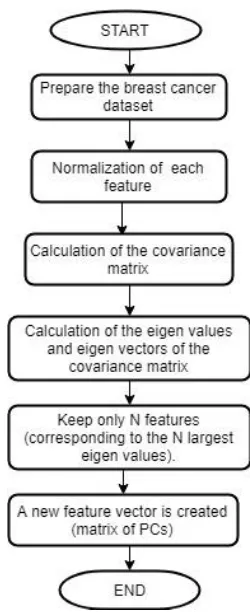
Figure 1. Flowchart of proposed algorithm.
This technique is widely used in the field of medicine for diagnosis of the disease. As dataset may have many such hyperplanes, SVM algorithm performs margin maximization which means that it tries to
create maximum gap between different classes [2]. In this dataset we observe the obscurity in classes. A simple line is unable to divide the Wisconsin breast cancer dataset into desired classes. The obscurity is seen in the figure 2.1.1.
Figure 2.1.1: Class Distribution in Wisconsin Dataset [2].
Figure 2.1.2: Classification using kernel[2].
2.2 PRINCIPLE COMPONENT ANALYSIS
PCA stands for principal component analysis; it is a tool that is used to identify patterns in data especially in which the data is dimensionally complex in nature. It was invented in 1901 by Karl Pearson. This tool converts a set of instances of variables that are possibly correlated to a set of instances of variables that are linearly uncorrelated called principal components. This conversion is done using orthogonal transformation. In this transformation, the largest possible variance belongs to the first principal component and each component that succeeds is said to have the highest variance value given that it has to be orthogonal to the components that precedes it [5]. The output is an orthogonal basis set which is uncorrelated in nature.
Experts in the field of machine learning use this tool for the preprocessing of data for their neural network; it is also used in exploratory data analysis and for constructing predictive models [9]. By centering the given input data then rotating and scaling it, this tool arranges the dimensions according to its priority allowing the elimination of some dimensions which has low variance. In this paper, PCA is implemented by Eigen value decomposition of data covariance matrix after the initial data is normalized. When the principle component has an Eigen value of zero, it signifies that it has’t explained
the variance present in the data, hence principal components with zero or near zero Eigen values are mostly discarded during dimensionality reduction [5]. This tool is sensitive to the scaling that is relative in nature of the original variables [6].
The main principle and goal of the principal component analysis is to reduce the feature of a dataset called dimensionality which contains many variables which are co related to each other while maintaining and retaining the spread and variation in the dataset [5]. Hence it is also called a dimension reduction tool that reduces huge set of instances to a small set that still contains significant information that was present in the huge set. This step improves the speed of convergence and the overall performance and quality of the neural network. To understand this tool, there are four basic statistical terms that has to be defined as their equations are related closely to each other [6].
They are: Mean, Standard deviation, Variance and covariance.
Mean :
This term is calculated by dividing the sum of all the instances present in the defined set X by the total number of instances in the defined set X given in equation 1. For instance, the mean height of students studying in a class will be the sum of each students height divided by the number of students in that class.
...(1)
Standard deviation :
……(2)
Variance:
This term measures the level of spread in data. For
instance the measurements of student’s heights
studying in high school won’t have a lot of variance since all of them can be categorized into the category of four feet and above whereas if the students of kindergartens heights are measured along with the high schooling students’ height, the value of variance will be higher. Hence variance signifies the amount or level of spread or difference in data. Variance is calculated by squaring the value of standard deviation given in equation 3.
..(3)
The difference value between the data points and the calculated mean becomes positive by squaring that value such that the values that lie above and below the calculated mean don’t cancel each other.
We take the age of a person on the x-axis and height of the person on the y axis generating an oblong scatterplot given below:
Figure 2.2.1: Scatter plot.
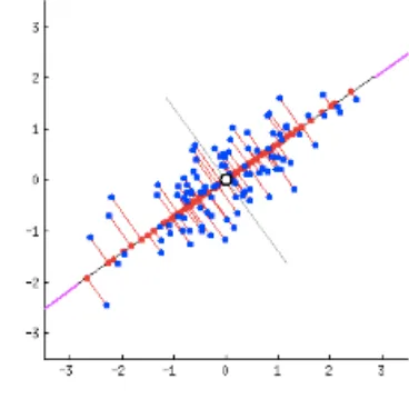
Principal component analysis like linear regression attempts to sketch a straight line, these straight lines through data are explanatory in nature [6]. Each and every line drawn through data represents a relationship between variables i.e. between a dependent variable and independent variable called principal component. Since there are as many lines as the number of dimensions in the given data, there are many principal components and the role of PCA is to prioritize them [7]. The bisection of a scatterplot is done by the first principle component with a straight line in such a manner that it signifies the most spread in the data. The bisection is shown below:
Figure 2.2.2: Scatter plot.
To fit the errors that were produced by the first principal component, the second principal component cuts the data perpendicular to the first component. Since there were only two dimensions in the graph above, they were only two principal components. If it were the data had been three dimensional, the third principal component would have fitted errors produced by second and first principal component and so forth.
III. EXPERIMENTS AND METHODOLOGIES
implementation is performed using scikit-learn which is an inbuilt library of Python. After importing SVM from sklearn, the dataset using the train_test_split function is divided into training set and test set as follows:
X_test, X_train, y_test and y_train
(where, X is a predictor and y is the target)
Creation of SVM classification object called SVC is performed which constitutes of various parameters which can be tuned according to the requirement. The parameters of SVC classifier are as follows [9]:
• C: It is a penalty parameter also called the regularization parameter. In the calculation of accuracy in this paper we have kept the value of C=0.5.
• Kernel: It determines the type to kernel to be used in the algorithm. It tends to be 'direct', 'poly', 'rbf', 'sigmoid', 'precomputed', or a callable. The default value is 'rbf' (Radial Basis Function). • Degree: It is given as the degree of the
polynomial kernel function. The default value is three and the same has been used in our paper. • Gamma: the coefficient of ‘rbf’ is given as gamma.
In the paper we have used the default value of
gamma which is ‘auto’.
• Coef0: The coef0=0 is used in the implementation
as it is insignificant in ‘rbf’. It’s value is the
independent term in the kernel function [10]. • Cache_size: It determines the size of the cache.
The cache_size=200 in our implementation. • Random_state: It is the pseudo random number
generator used for shuffling the data.
• Max_iter= -1, which species no hard limit on the number of iterations. Negative one, is the default value and also the one used in our paper.
Then, we fit our model on training dataset and perform prediction on the testing dataset using fit() and predict() respectively. Accuracy is then computed by comparing the predicted values with
the test dataset values. The accuracy achieved in our implementation is 95.1%. We have improved the accuracy of SVM classifier using the following series of steps:
3.1 Using the min-max scaling
Most of the times, the dataset will contain exceptional fluctuations in magnitude, units and range. Be that as it may, since, the greater part of the machine learning algorithms use Euclidian distance between two information focuses in their calculations, this is an issue [11].
The accuracy of training dataset using the SVM classifier came out to be 100% without the use of min-max scaling which is also called normalization. This was due to the overfitting of the training dataset. To overcome overfitting and also to suppress the outliers, normalization is brought into use. It can be avoided by limiting the absolute value of the parameters in the model. This can be done by adding a term to the cost function that imposes a penalty based on the magnitude of the model parameters. This scaling technique bounds the features between a maximum and a minimum value, which is often between zero and one. This has been achieved by using the MinMaxScaler. The use of this estimator will result into negligible entries in sparse data.
The formula [12] of Min-Max scaling is given in the equation 4:
…..(4)
This scaling bounds the value between 0 and 1.
3.2 Using feature selection technique called PCA
This feature selection technique is a statistical method to draw out concealed features from multidimensional data [13]. This is the transformation which involves compression of dataset using linear algebra. Application of PCA in the Wisconsin Diagnostic Breast Cancer dataset improved the accuracy of the test dataset from 95.1% to 96.5%. Working of PCA is illustrated in Figure 3.1.1.
Step1: Prepare the dataset. Create a matrix which accommodates all the features of the Wisconsin Breast Cancer dataset.
Step2: We perform normalization of the features by subtracting the mean from each dimension to produce a dataset having null mean. Post normalization, each predictor has mean equal to zero and standard deviation equal to one as given in equation 5.
….(5)
Where, xi indicates the various features of the dataset
and denotes the mean of the dataset. Normalization is a necessity as the original features may have varying scales. If PCA is performed on the un-normalized predictors then then the new feature vector will only contain variables with high variance. Principle component will completely be dependent on the variables with high variance and this is an issue. For example: If there are three nodes, namely A, B and C. The distance between the node A and B is given as 5000 m and the distance between the node B and C is 5 km. The variance of the distance between node A and B will be much higher than the variance of the distance between the nodes B and C. Therefore, it is really important to bring all the predictors on uniform scale.
Figure 3.1.1: Working of PCA.
Step3: After normalization, the covariance matrix is computed. This matrix gives the description of the variance of the data and also depicts the covariance among variables. It gives an empirical description of the data. The covariance matrix is formulated using the formula in equation 6 -
..(6)
The diagonal elements store the variance of the principle components. If the non-diagonal elements of the covariance matrix are positive, it implies that the variables X and Y will increase together. Otherwise, when the variable X increases, the variable Y will decrease.
Step5: The next step is to arrange the Eigen values in the decreasing order as given in equation 7 –
……(7)
The feature with largest Eigen value is the principle component of the dataset. In our implementation of Wisconsin Breast Cancer Dataset, we have kept the threshold to one. All the features with Eigen value greater than one are kept whereas others are omitted.
Step5: A new feature vector is created which comprises of all the principle components of the dataset. The dimension of the dataset has been reduced and now it only contains those features which capture maximum information and are not co-related with one another.
IV.DATASET
The training data set that has been used in this paper has been taken from the Wisconsin Breast Cancer Data. This dataset is present in the open source repository called the UCI Machine Learning [15]. This data set is multivariate and has over 569 instances. There are over ten features that describe the cell nuclei whose digital image is taken to classify it as malignant or benign. The Ten attributes are between the center and perimeter.
viii) Smoothness: local disparity in the length of radius.
ix) Symmetry
x) Texture: S.D of gray-scale values, where S.D stands for Standard Deviation.
V. SIMULATION SOFTWARE
In this paper, the Anaconda software was used as the machine learning tool. Anaconda is a python based open source tool that was first released to the public in 2012 under the New BSD License. It provides several machine learning algorithms and techniques including the algorithms that are being studied in this paper.
Anaconda is a free and open-source distribution of the Python and R programming languages for scientific computing .The features of this software also include data science, large-scale data processing and predictive analytics.
VI.DISCUSSION
This section describes the parameters and sets forth the result of six different machine learning techniques that are being explored in this paper.
A. Accuracy exceedingly dependent upon the threshold used in the classifier [17].
The accuracy can be calculated as:
Accuracy = (TP+TN)/(T+P) ……..(5)
P is positive and it signifies the cancerous cells i.e. malignant whereas N stands for Negative and represents the noncancerous cells i.e. benign.
B. Recall
The definition of recall is given as the rate of True positive instances and False Negative instances that have been classified as True Positive. This measure is used in the medical field as it gives knowledge about the number of cases that are correctly identified either as malignant or as benign. It is the ability of the model to find all the relevant cases in the dataset.
The recall can be calculated using the Equation 8 [17]:
Recall = TP/(TP+FN) …….(8)
C. Precision
Precision is also called confidence. The definition of precision is given as the rate of True Positive instances and False Positive instances that have been classified as True Positive. Precision shows the ability of the classifier to handle the positive instances; it does not say anything about the negative instances. Recall and precision share an inversely proportional relationship with each other [18]. This parameter can be calculated using the equation 9 [19]:
Precision = TP/ (TP+FP) ……….(9)
VII. RESULT ANALYSIS
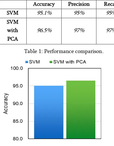
The table 1 given below shows the calculated accuracy, recall and precision of support vector machine algorithm before and after the application of principle component analysis.
In the figure 7.1 shows the comparison of accuracy achieved using SVM and PCA/SVM via a bar chart.
Accuracy Precision Recall
SVM 95.1% 95% 95%
SVM with PCA
96.5% 97% 97%
Table 1: Performance comparison.
Figure 7.1: Accuracy Comparison.
VIII. CONCLUSION
Support vector machine algorithm can be used to predict breast cancer with an accuracy of 95.2% and this accuracy can be further improved by applying a feature selection method called the Principle component analysis. The improved accuracy of the algorithm is 96.5%. Hence, SVM along with PCA can be used to develop and automate systems that would predict breast cancer in patients overcoming time consuming procedures that were conducted manually leading to a decrease in diagnostic test fees as well as in diagnostic errors.
IX. REFERENCES
[2]. D. Parkin, “Epidemiology of cancer: global patterns and trends” Toxicology Letters. vol. 5,
pp. 102-103, 1998.
[3]. Meriem Amrane, Saliha Oukid, Breat Cancer Clasification,Using Machine Learn-ing, Proceedings of 2010 IEEE Student Conference on Research and Development (SCOReD 2010), 13 - 14 Dec 2010,Malaysia.
[4]. R. Setiono, “Generating concise and accurate
classification rules for breast can-cer diagnosis”
Artificial Intelligence in Medicine. vol. 18, pp. 205-219,2000
[5]. Subhagata Chattopadhyay,”A neuro-fuzzy
approach for the diagnosis of
de-pression”,Applied Computing and Infor-matics Volume 13, Issue 1, January 2017
[6]. https://skymind.ai/wiki/eigenvector
[7]. K. Kourou, T. P. Exarchos, K. P. Exarchos, M. V. Karamouzis, and D. I. Fotiadis,“Machine
learning applications in cancer prognosis and
prediction,” Comput. Struct.,Biotechnol. J., vol.
13, pp. 8-17, 2015.
[8]. Noushin Jafarpisheh, Nahid Nafisi “Breast
Cancer Relapse Prognosis by Clas-sic and Modern Structures of Machine Learning
Algorithms” 2018 6th Iranian Joint Congress on
Fuzzy and Intelligent Systems (CFIS)
[9]. Rohit Arora and Suman "Comparative Analysis of Classification Algorithms on Different Datasets using WEKA," 2012 International Journal of Computer Applica-tions (0975 - 8887) Volume 54- No.13, September 2012. [10]. Yu-Len Huang, Kao-Lun Wang “Di-agnosis of
breast tumors with ultrasonic texture analysis using support vector ma-chine” Neural Comput
& Applic (2006) 15: 164–169 DOI 10.1007/s00521-005-0019-5
[11]. A. Soltani Sarvestani, A. A. Safavi “Predicting
Breast Cancer Survivability Using Data Mining
Techniques” 2010 2nd International
Conference on Software Technology and Engineering(ICSTE)
[12]. Runjie Shen, Yuanyuan Yan, “Intelli-gent Breast Cancer Prediction model using data mining techniques”, 2014, 6th Interna-tional Conference on Intelliegent Human machine system & Cybernetics, Tongji University Shanghai, China.
[13]. Subhagata Chattopadhyay “A neuro-fuzzy approach for the diagnosis of de-pression”
Department of Computer Sci-ence and Engineering, National Institute of Science and Technology, Berhampur 761008, Odisha, India. [14]. Liton Chandra Paul, Abdulla Al Sumam, “Face
Recognition Using Principal Component
Analysis Method” Interna-tional Journal of Advanced Research in Computer Engineering & Technology (IJARCET) Volume 1, Issue 9, November 2012.
[15]. M. Lichman, UCI Machine Learning Repositry,
2013. Online].
Availa-ble:https://archive.ics.uci.edu/.
[16]. Boulehmi Hela, Mahersia Hela, Ham-rouni Kamel, Breast Cancer Detection ,AReview On Mammograms Analysis Techniques, 2013 10th International Multi-Conference on Systems, Signals & Devices (SSD) Hammamet, Tunisia.
[17]. 2014 IEEE 10th International Collo-quium on Signal Processing & its Ap-plications,(CSPA2014), 7 - 9 Mac. 2014, Kuala Lumpur, Malaysia
[18]. G. Williams, “Descriptive and Predic-tive
Analytics”, Data Min. with Ratt. R Art,Excav.
Data Knowl. Discov. Use R, pp. 193-203, 2011. [19]. Muhammad Sufyian Bin Mohd Azmi,Zaihisma
Che Cob,”Breast Cancer Prediction Based On
Backpropagation Al-gorithm ”,Proceedings of 2010 IEEE Stu-dent Conference on Research and Devel-opment (SCOReD 2010), 13 - 14 Dec 2010,Putrajaya, Malaysia.
[20]. Mandeep Kaur, Rajeev Vashisht “Recognition
Decomposition” International Journal of Computer Applications (0975 – 8887) Volume 9– No.12, November 2010
Cite this article as :
![figure 1.1 [20]](https://thumb-us.123doks.com/thumbv2/123dok_us/1048628.1131074/2.595.318.547.177.335/figure.webp)
![Figure 2.1.2: Classification using kernel[2].](https://thumb-us.123doks.com/thumbv2/123dok_us/1048628.1131074/3.595.53.276.75.223/figure-classification-using-kernel.webp)