Intersection Control as a Shared Decision Process.

ABSTRACT

ISUKAPATI, ISAAC KUMAR. Intersection Control as a Shared Decision Process. (Under the direction of Dr. George F. List).

This research introduces a novel way to develop a signal control strategy in which drivers

(figuratively and literally) play an active role in making control decisions. A bid-based

control strategy is proposed to explore these ideas.

In the proposed framework there are high and low value-of-time drivers that interact with

movement managers by paying compulsory and voluntary fees to reduce their delays. The

movement managers, one for each turning movement, place bids for control of the

intersection. A municipality receives the bids and decides which movement managers win.

First-price bidding is employed. The thesis describes what these players do, how they

interact, influence of data availability on how they behave, and how their decisions influence

the resulting signal timings.

To facilitate the examination of these ideas, an agent-based simulation model of the strategy

is created in Python. The simulation model involves an intersection involving two single-lane

one-way streets with a total intersection volume held constant at 1500 veh/hr/lane. The

analysis for three traffic flow combinations is presented. For a given input volume on the

facility, the program creates a sequence of arrival headways for both approaches. The arrival

headway distribution is generated from a shifted negative exponential distribution with a

minimum headway of 1.5 seconds and an average headway consistent with the arrival flow

rate. A Python-based model of actuated control is also developed for the purposes of

benchmarking the analysis. These two simulation models exist within the same analysis

program.

Creation of the simulation model illustrates that fact that signal control strategies can be

© Copyright 2014 by Isaac Kumar Isukapati

Intersection Control as a Shared Decision Process

by

Isaac Kumar Isukapati

A dissertation submitted to the Graduate Faculty of North Carolina State University

in partial fulfillment of the requirements for the degree of

Doctor of Philosophy

Civil Engineering

Raleigh, North Carolina

2014

APPROVED BY:

_______________________________ ______________________________

Dr. Alain L. Kornhauser Dr. Alan F. Karr

(Princeton University) (UNC Chapel Hill)

_______________________________ ______________________________

DEDICATION

Were the whole realm of nature mine;

That were an offering far too small;

Love so amazing, so divine;

Demands my soul, my life, my all….

I dedicate this thesis first to the Glory of my maker and savior Lord Jesus Christ, and then to

BIOGRAPHY

Isaac Kumar was born in India and received Bachelors of Engineering from Andhara

ACKNOWLEDGMENTS

 Thanks to my parents and extended family: especially want to thank my dad, late mom,

my dear brother Philip, and his wife Shivani for supporting me throughout the process

 Thanks to Dr. List for being a caring and insightful mentor. I am deeply indebted to him

for shaping me the researcher that I am today. You are epitome of what an ideal advisor

 Thanks to my committee members for their continued guidance. I specially want to thank

Dr. Kornhauser, and Dr. Karr for their insights

 A special thanks to Dr. Hoon Hong for his wise counsel whenever I needed it

 Thanks to Raja aunty & Uncle John for their continued support. Both of you are very special to me

 Thanks to Andy & Erica Owens for the care that you showed towards me when I was in

the hospital

 Thanks to Dr. Richard Chulie for caring and praying for me when I was in the hospital. I

am deeply indebted to you

 Thanks to my friends in graduate school Naresh, Sashi, Shalini, Venu, Senganal,

Fatemeh, Sarah & Yuriy; a special thanks to Sashi, and Yuriy for the long drives and philosophical conversations at 1 AM

 Thanks to Ajay & Prasanna for your support and the beautiful fellowship that we share

 Thanks to Ajay Kumar for showing me how amazing computer science actually is

 Thanks to John & Sharyn Gibson – both of you are very special. John thank you for the

conversations that I had with you (music, theology, technology, engineering, history just to name a few).

 Thanks to Danielle, Anna and Vasek for all our nerdy conversations.

 Thanks to IBS family: Mrs. McGee, Kosobucki’s, Whites, Stevens, Jenkins (Chase & Laura both of you are amazing)

 Thanks to Jenn & Ani for all the good times we had

 Thanks to FBC church family for the wonderful fellowship that I had there

 Thanks to Steve Edwards for his constant encouragement, exhortation, and other nerdy conversations. You are special dear brother!

 Thanks to Emmy, Teddy, Amy & Ivan Kandilov for the love that you showered upon me.

Both of you are very special to me; a special thanks to my little buddy “Emmy” for playing with me whenever I needed a break.

 Thanks to Justin, Matt & Sijy Abraham for your wonderful friendship. Three of you are

TABLE OF CONTENTS

LIST OF TABLES ... viii

LIST OF FIGURES ... ix

CHAPTER 1: INTRODUCTION ...1

1. Introduction ...1

1.1. Problem Motivation ...1

1.2. Problem Formulation ...2

1.3. Research Contributions ...2

1.3.1. Bid Based Control Strategy ...3

1.3.2. Agent-based control ...3

1.4. Document Organization ...3

CHAPTER 2: RELATED RESEARCH ...4

2. Introduction ...4

2.1. Market-inspired ideas applied to traffic signal control ...5

2.2. Classic control strategies for isolated intersections ...7

2.2.1. Fixed-Time Control ...7

2.2.2. Actuated Control ...7

2.2.3. Adaptive Control ...8

2.3. Conclusions...9

CHAPTER 3: METHODOLOGY ... 10

3. Intersection Control in a Game-Like Structure ... 10

3.1. Description of the players ... 11

3.3. Realizations of the game ... 14

3.4. Bidding strategies ... 15

3.4.1. State-observer systems ... 15

3.4.2. Probabilistic systems ... 16

3.5. Summary ... 16

CHAPTER 4: A REALIZATION OF THE GAME ... 17

4. Introduction ... 17

4.1. Player Details ... 17

4.1.1. Movement managers ... 17

4.1.2. Drivers ... 20

4.1.3. Municipality ... 25

4.2. Flowchart for the Game Logic ... 28

4.3. Actuated Control Model ... 30

CHAPTER 5: SIMULATION EXPERIMENTS AND ANALYSES ... 32

5. Introduction ... 32

5.1. Simulation experiments ... 32

5.2. Setting the saturation headway distribution... 34

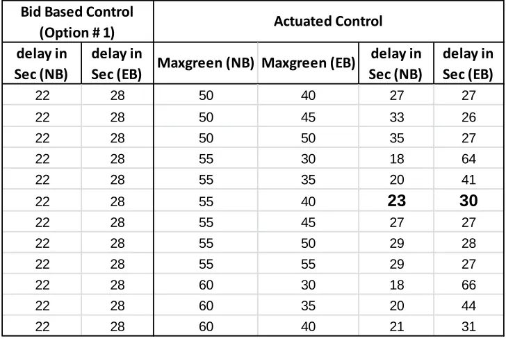
5.3. Setting the maximum greens ... 35

5.4. Consistency among Simulations ... 37

5.5. Evaluation and analysis ... 39

5.5.1. CDFs of individual vehicle delays ... 40

5.5.2. CDFs of cycle lengths ... 44

5.5.4. Impact of queue length on bids ... 51

5.5.5. Income stream received by the municipality ... 53

5.6. Variations in the driver contributions... 53

5.6.1. Analysis of Results ... 55

5.7. Summary ... 68

CHAPTER 6: CONCLUSIONS AND FUTURE WORK ... 70

6. Concluding Remarks... 70

6.1. Bayesian Game ... 71

6.2. Explore auction theory concepts ... 73

6.3. Explore information theory concepts ... 74

6.4. Explore other classes of bidding systems ... 75

6.5. Develop a game for more approaches ... 75

REFERENCES... 76

APPENDICES ... 83

APPENDIX A ... 84

LIST OF TABLES

Table 1: Table of possible voluntary contributions ... 24

Table 2: Average delay (sec) for different combinations of maxgreen for Scenario-2 flow condition ... 36

Table 3: KS Test results to check consistency among simulations ... 39

Table 4: KS Test results for delay distributions for NB ... 41

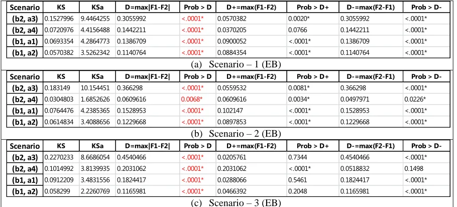
Table 5: KS Test results for delay distributions for EB ... 41

Table 6: Various delay statistics for six simulation options ... 44

Table 7: Summary of KS Test results for distribution of average payments... 48

Table 8: Summary statistics of delays for two classes of drivers ... 48

Table 9: summary of driver payments vs cost of service ... 49

Table 10: summary of average driver payments vs average cost of service ... 50

Table 11: Results of t-Test to check differences in cost of service ... 50

Table 12: Total funds ($) transferred to the municipality per hour ... 53

Table 13: Summary of KS test results (delay) ... 58

Table 14: Voluntary contribution statistics for seven cases ... 60

Table 15: Voluntary contributions made by drivers with a low value-of-time ... 60

Table 16: Voluntary contributions made by drivers with a high value-of-time ... 60

Table 17: Additional income contributed by two classes of drivers ... 62

Table 18: Summary of KS Test results individual payments ... 64

Table 19: Average cost of service ... 65

Table 20: Summary of KS Test results win bids ... 67

LIST OF FIGURES

Figure 1: Representation of the overall system... 10

Figure 2: Computing the selected bid... 19

Figure 3: Schematic of driver j’s decision network ... 23

Figure 4: Schematic showing cost of incremental delay ... 26

Figure 5: Flowchart for the control structure of the simulation model ... 30

Figure 6: CDFs of individual vehicle delays in ten simulation runs ... 38

Figure 7: Results (delays) for six simulation scenarios (NB) ... 43

Figure 8: Results (cycle lengths) for six simulation scenarios ... 45

Figure 9: Cumulative density functions of various payments ... 47

Figure 10: Probability Density Functions (PDFs) of bid amount for various queue lengths .. 52

Figure 11: CDFs of individual vehicle delays ... 56

Figure 12: CDFs of voluntary contributions ... 59

Figure 13: CDFs of individual vehicle payments ... 63

CHAPTER 1: INTRODUCTION

1.

Introduction

The role of economics is instrumental in transportation decision making. However, only in

recent years, have competitive market ideas been proposed as a paradigm for controlling

urban road traffic systems (68-70). In this research, auction based principles and a paradigm

akin to a game (but not derived from game theory) is used to create a signal control strategy.

That is, instead of using the standard techniques of minimum greens, maximum greens, and

gaps to control the signal indications, an economically based game structure is employed.

The intersection’s space is viewed as a scarce commodity whose use is determined through a

bidding process. Movement Managers oversee the vehicle departures for specific turning

movements. Arriving motorists pay the Movement Managers to arrange times of entry for

them. Movement Managers submit bids for use of the intersection’s space and the highest

bidders win. Distributed processing and connected vehicle technology (1-8) are the

mechanism by which implementation would be feasible. The value of these ideas is that one

can study the economics that underlie the control.

1.1.

Problem Motivation

Doctoral research focuses on new ideas, and finding creative solutions to important societal

problems. One such problem is traffic signal control. The evolution of this field in the last

several decades has been significant. It has progressed from simple fixed-time control to

actuated control and distributed control. Control and systems engineers have advanced the

state-of-the-art and state-of-the-practice based on their domain knowledge of instrumentation

and control.

An interest in both agent-based modeling and traffic signal control motivated this research to

study signal control from the perspective of economic theory. While the topic can clearly be

pursued from the perspective of intellectual curiosity, it is possible today to picture how it

where it is reasonable to think about signals talking to vehicles and vice versa. An extensive

body of research that focuses on use of these technologies is enhancing both observability

and the safety of transportation networks (1- 8).

Philosophers share a common interest with economists in the sense of maximizing human

welfare. In addition, philosophers are concerned with logical justification of actions with

respect to their expected outcomes. The thesis that underpins this proposed research is that a

control strategy created based on auction theory principles would provide interesting insights

into the costs of delay at a signalized intersections and aide our understanding of how to

make investment decisions.

1.2.

Problem Formulation

The processing space of an intersection is viewed as a scarce commodity. In that sense, one

can look at that commodity from an economic perspective and determine how to allocate its

use, but to the best of this author’s knowledge, this has not been done. Rather, the use of this

commodity in time and space has been studied through system engineering concepts related

to control theory: determining what movements should be allowed to move when, for how

long, to optimize performance measures such as delay, queues, stops etc. The advent of V2I

makes it possible to consider the control problem from an economic perspective: having the

users pay to get responsive treatment. The expectation is that such ideas will produce

solutions that are different from those obtained today; solutions whose economics is

understood. So, this research proposes to investigate the ways of creating signal control

strategies using auction theory principles.

1.3.

Research Contributions

1.3.1. Bid Based Control Strategy

This research has introduced a novel way to develop a signal control strategy that is based on

economic considerations. The control strategy creates signal timing plans whose economics

can be understood.

1.3.2. Agent-based control

An agent-based model of intersection control is presented. Using a game-like setting,

movement managers (computer applications) bid for green time on behalf of vehicles

associated with specific turning movements. The movement managers also collect fees from

arriving vehicles, determine what those fees should be, and strive to minimize the delays for

their constituents while not charging more than the minimum required to do so. In each turn

of the game, winning movement managers discharge a single vehicle from the front of their

queues. An additional entity (e.g., a municipality) oversees the game and manages the

bidding process.

1.4.

Document Organization

Chapter 2 reviews related literature focusing on resource allocation as well as isolated

intersection control. Chapter 3 provides overview of the methodology. Chapter 4 presents a

detailed discussion on how to create a realization of the game. Chapter 5 presents details on

simulation experiments and analysis; Chapter 6 provides concluding remarks and future

CHAPTER 2: RELATED RESEARCH

2.

Introduction

Resource allocation problems deal with the assignment of resources to activities and the

scheduling of those activities. For example, resource allocation pertains to the allocation of

landing slots at airports, workstations in job shops, CPU time slices for computers, and beds

and medical personnel in healthcare facilities. Moreover, simulation-based games offer a way

to study these problems.

The allocation of intersection space through signal control is a problem to which resource

allocation techniques can be applied. The signal control can be seen as a process that assigns

intersection space (the resource) to vehicles. It does this by separating the intersecting vehicle

movements in space and time. These separations are manifest in the phase sequences and

switching times. (Here, a phase is considered a combination of movement greens that occur

simultaneously, as would be the case with simultaneous eastbound and westbound left turns.)

Ostensibly, the switching strategy is not only safe but efficient. Not only can intersection

control be viewed as a resource allocation problem, but it can also be seen as a game in

which a shared decision process among various players determines the phase sequence and

switching times.

Ideas from competitive markets and multi-agent systems can be used to create the models of

such control systems. Hence, this review of related research focuses on instances in which

market-inspired approaches or multi-agent systems have been applied to traffic signal

control. Furthermore, the research’s focus on isolated intersection control makes it necessary

to review prior work in that area, but not for network control. Readers interested in network

signal timing strategies can find comprehensive reviews in (9-32).

While the agent-based simulation model created in this doctoral work is not technically

work in this domain. These efforts helped shape the ideas upon which the simulation model

is based. Game theory is the branch of mathematics that focuses on studying strategic

interactions among various players. The players often want to maximize their own success in

response to the strategies used by the other players in the game. Game theory pertains to

many situations. Resource allocation is one of them. For example, Grether et al. (72) use

game theory to study the allocation of landing rights. Adler (73) presents a two-stage

game-theoretic framework to solve the landing slot-allocation problem. Chang et al. (74) use

cooperative and non-cooperative game mechanisms to study the bandwidth allocation

problem in wireless networks. Ahmad et al (75) use game theory for scheduling tasks on

multicore processors. McMillan (76) use an auction-based game to study the sale of radio

spectrum rights. Zhou et al. (77) propose a game theory-based approach to study job

scheduling in networked manufacturing. Kutanoglu, Wu (78) apply a combinatorial auction

to solve a distributed resource scheduling problem. Li et al. (79) use cooperative gaming to

automate the process of planning and scheduling.

2.1.

Market-inspired ideas applied to traffic signal control

In recent years, researchers have begun applying agent-based techniques to traffic control.

Agent-based control involves using distributed intelligence, often autonomous, to develop

problem solutions. For example, Choy et al. (80) present a cooperative, hierarchical,

multiagent system for real-time traffic signal control. The control problem is divided into

sub-problems, and each sub-problem is handled by an intelligent agent that makes decisions

using principles from fuzzy-neural networks. The decisions made by lower agents are

mediated by higher level agents. This means the multi-agent system is hierarchical.

Agent-based systems often use learning techniques to adapt to the evolving traffic conditions.

For example, Steingrover et al. (81), Weiring (82) employ a reinforcement learning technique

to minimize the overall waiting time of the vehicles. Here the learning task is represented as

Some researchers suggested adapting market-based ideas to traffic signal control. For

example, Dias et al. (83) suggest a market-based coordination mechanism for signal

coordination. These mechanisms are analogous to the functioning of commodity markets.

The agents that regulate the infrastructure act as a team to achieve a desirable solution.

Schepperle and Bohm (84) proposed an auction-based policy for intersection control. Here,

the intersection control agent starts an auction for the earliest departure time slot among the

vehicles that are approaching the intersection on each lane. Only the lead vehicle in each

queue is allowed to participate in the auction.

Similarly, Vasirani and Ossowski (69, 70) propose a multiagent approach to design a

competitive computational market for the distributed allocation of an urban road network. In

specific, they propose intersection manager – driver model in conjunction with cooperative

learning techniques to coordinate the prices of individual intersections. This framework uses

walrasian auction system for selling intersection schedule slots. Basically walrasian auction

involves a set of buyers and a set of suppliers. At a given time, each buyer in the set of

buyers notifies the suppliers the quantity of resources he/she going to buy at a preset

published price. Intersection manager in turn uses this information to compute total demand

and excess demand. Using this information the model updates intersection reserve prices

(reserve prices are upward adjusted in case of excess demand and downward adjusted in case

of excess supply). Drivers choose routes based on their own preferences between time and

cost, participating in intersections auctions as long as they are willing to meet the reserve

price. So, in that sense the intersections that drivers pass through are a function of their

willingness to pay the preset price for using those intersections. Although the research work

conducted in this thesis bears some similarity to this approach, there are some key

distinctions. Firstly, the game-like framework proposed in this research does not constrain

drivers from using the intersection space by setting undesirable costs of service. It rather

imposes an initial fee on all drivers (this is to cover marginal costs of operating the signal)

and enables drivers to make decisions about voluntary contributions to help expedite their

system, i.e., every driver that passes through the intersection influences the performance of

the signal. Thirdly, this doctoral work generalizes the notion of auctions subjected to

constraints set by traditional signal control theory (use of minimum greens, gaps, clearance

intervals) whereas intersection managers proposed by Vasirani et al., control the decision

nodes of an O-D in an urban network. Therefore in that sense these managers do not directly

influence the operations at a signalized intersection.

2.2.

Classic control strategies for isolated intersections

Inasmuch as the focus of this research is on signal timing for intersections, it is important to

review more classic control strategies. These methods can be placed in three categories: 1)

fixed-time control, 2) actuated control, and 3) adaptive control. A brief discussion of each is

presented below.

2.2.1. Fixed-Time Control

In fixed-time control a pre-determined phase sequence is combined with fixed green times

(and inter-green times). The same signal timings repeat from one cycle to the next.

Obviously, fixed-time control is unresponsive to any variations in demand that emerge from

cycle to cycle. The signal timings may vary across the course of a day, but that is because a

sequence of fixed timing plans is selected from a family of predetermined plans that are

developed off-line on the basis of historical traffic data (37).

2.2.2. Actuated Control

Actuated control uses detector inputs to determine the green time durations. Movement

sequences run in parallel, called rings, and they resolve the spatial conflicts. The ring

structure ensures that movements end simultaneously to ensure that spatial conflicts do not

arise. Green time durations are determined by minimum greens, gap timers, and maximum

greens. The resulting phase patterns (movement combinations) and switching times are

Actuated control can further be classified into fully-actuated control and semi-actuated

control (39). We discuss fully-actuated control here. Semi-actuated control pertains to

actuated signals in coordinated networks, and this paper does not focus on that domain.

In fully-actuated control, detectors are placed on all of the movements, upstream of the

stop-bar. The detectors identify the passage or presence of vehicles. The detector inputs enable the

signal controller to create phase sequences (movement combinations) and switching times

that are response to the traffic streams. Typically, a minimum green is followed by gap

timing; and if a gap timer reaches a maximum, which means a minimum headway has been

exceeded, the green time ends. In some cases, the minimum green time is variable. Time is

added if vehicles arrive while the signal is red. In volume-density control, the maximum

allowable gap reduces linearly after a prescribed amount of green time has elapsed. The

green also ends if a maximum green is reached.

Although actuated control works well, it has two major drawbacks. The first is that the phase

sequence options are restricted by the ring definitions. The controller does not have the

option to switch without restraint from one movement combination to another. The second is

that queue length does not influence decisions about whether or not to stop the extension of

green. The green time decisions are made strictly on the basis of gap sizes and minimum and

maximum greens. For example, at an intersection where the flow of traffic on various

approaches is significantly different, vehicles on the approaches with lower flows may

experience high delays. This is due to lack of opportunities for gap-out on approaches with

higher flows. Thus, it can be inferred that when traffic demand is heavy on all approaches,

actuated control may not produce the best performance (38).

2.2.3. Adaptive Control

Adaptive control is a hybrid strategy. The phase sequences and the switching times are based

deciding whether to continue green for the current phase or to switch to a different phase.

However, the detectors are not always linked directly to the movements, so the green times

are not necessarily determined by minimum greens, gaps, and maximum greens. The phase

durations can vary from one cycle to the next. Because the phase sequences can be changed,

adaptive control has an ability to outperform both pre-timed and actuated control. Examples

of adaptive control include MOVA: Microprocessor Optimized Vehicle Actuations (40-44),

CRONOS: ContROl of Networks by Optimization of Switchovers (45, 46) and SPPORT:

Signal Priority Procedure for Optimization in Real Time (47-49), OPAC: Optimized Policies

for Adaptive Control (50-53), COP: Controlled Optimization of Phases (54), PRODYN:

Programmation Dynamique (55-57), SCOOT (58), and SCATS(59). Descriptions of each of

these can be found in Appendix B.

2.3.

Conclusions

This chapter has presented an overview on family of resource allocation problems and

provided a few references on prior attempts to apply agent-based modeling ideas to explore

such problems. Furthermore, since the focus of this research is traffic signal control, an

overview of existing approaches to signal control at isolated intersections and/or agent-based

control. Most of the control system strategies for isolated intersections are based on systems

engineering concepts that pertain to control theory, but not economic theory. However, in

recent years, competitive market ideas have been proposed for controlling urban road traffic

CHAPTER 3: METHODOLOGY

3.

Intersection Control in a Game-Like Structure

As mentioned earlier, the intersection control problem is treated here in a game-like fashion

where there are movement managers (figuratively and literally) that negotiate for use of the

intersection on behalf of the drivers making a specific turning movement. This means at a

typical four-leg intersection there would be eight movement managers: four for the

through-and-right movements; and four for the left turns. The outcome is a sequence of wins, for

specific movement managers, which translates into vehicle discharges by movement. In

effect, playing the game creates the signal timings.

Figure 1: Representation of the overall system

As presented in Fig. 1 the game-based formulation has two worlds that evolve in parallel.

The first is the physical system. The second is the game. The game outcome affects the

Physical (Traffic) Bidding (Economics)

Overall System

Dynamics of the System

physical system and vice versa. Game results determine what vehicles get to be discharged,

and those discharge events affect the bidding decisions of the movement managers.

3.1.

Description of the players

The players in the game are as follows:

Drivers: Drivers are players who travel through the network. They arrive at the intersection

because it is in their path. They want to pass through the intersection in minimum time.

Drivers can be either active or passive players in the game. If they are passive, then they pay

the movement manager to arrange a time for them to go and then they wait for their

appointed entry time. On the other hand, if they are active players, they constantly evaluate

the system, and take actions to expedite their service.

Movement Managers: Movement managers are players who bid against one another for use

of the intersection. When they win, they release motorists from their waiting queue. They

develop bidding strategies that maximize the likelihood of their winning. The bidding

strategies can be developed either from principles of probability theory or state-observer

systems. They collect fees from their drivers and then pay the municipality for the use of the

intersection. Movement managers have “bank accounts” into which they deposit payments

from the drivers and from which they pay the municipality.

The Municipality: The municipality is the player that oversees the game. It manages the

bidding process and determines which movement manager(s) win. The municipality also

ensures that scarce societal resources are utilized optimally. In addition, the municipality

creates the game and its rules.

3.2.

Game Terminology

As with any game, rules govern how the game is played, and the relationships among the

A time step is the increment by which the game proceeds. In the context of this discussion,

the time step is 0.1 seconds. The state of the game is updated for every 0.1 seconds.

A discharge slot is an increment of time allocated for discharging a single vehicle; presently,

it is 2.1 seconds. This value is chosen because it is typical saturation headway between

vehicles being discharged at the stop bar.

An initial fee is the amount paid by arriving motorists to their respective movement mangers

upon their arrival.

A nominal fee is the minimum cost for using the intersection.

Enfranchised manger is the movement manager that currently holds the intersection control.

Disenfranchised manager is the movement manager that doesn’t hold intersection control

currently, but is competing for it.

Delay is the additional time that drivers incur if their movement manager loses the current

bid event.

Marginal cost of delay is the marginal cost associated with the delay.

Financial transactions occur between the movement managers and the travelers or

movement managers and the municipality. The movement managers charge an initial fee to

the travelers. Movement managers pay the municipality for discharging their vehicles –

either what they bid – if they win a bid – or a nominal fee if no competitive bid takes place

(because no other movement manager had vehicles wanting to use the facility in a particular

discharge slot). The financial transactions also occur during each turn, subsequent to the

between the movement managers and the travelers and movement managers and the

municipality.

Each movement manager has a bank account into which payments by the drivers are placed

and from which payments to the municipality are made. Each movement manager monitors

the balance in her/his account to ensure that it remains solvent.

Events are the actions that take place during the game. Three events take place in each time

step. The first is the bid. The bidding determines how the intersection is used in the next

discharge slot. The second is one or more financial transactions. Effectively, time “stands still” while these two events take place. The third event is the “vehicle release”. It takes place

once discharge slot(s) have been assigned to specific movement manger(s). The vehicles then

pass through the intersection. As indicated above, for any given movement, one vehicle per

lane can be released on any given movement during a single discharge slot.

A turn of the game encompasses these three events: the bidding followed by the financial

transactions, and then the vehicle discharge(s). Each turn ends when the “business” of the

turn is completed: the transactions between the winning movement manager(s) and

municipality are finished, the winning movement manager(s) have discharged their first

vehicles in queue; the system information is updated, and the players are ready to participate

in the next turn of the game. This process continues until the game ends (which is at the end

of the analysis period).

A performance metric is a measure used to assess the quality of the signal control.

Consistent with conventional practice, delay is used. Early ideas about delay were developed

by Wardrop, (33) and analytic expressions for the delays were later presented by Webster

(34, 35) and Newell (36) provides additional thoughts about the manner in which delay can

3.3.

Realizations of the game

The concepts presented above must be translated into a specific realization of the game in

order for the game to be played. A given realization is defined by: 1) the rules by which the

game is played, 2) the bidding strategies, 3) the objectives being pursued by the players, and

4) the information being shared.

The rules determine how the bidding process takes place, the manner in which the movement

managers can interact with one another, the amount of information shared with the bidders.

For instance, the municipality gets to decide whether the bidding process is single-stage or

two-stage. In addition, the municipality decides how much the winning movement managers

pay: two examples are their bid amount (first price sealed bidding) or the amount bid by the

second highest bidder (second price sealed bidding).

The bidding strategies determine how the movement managers develop their bids and what

information they have when they do that. The movement managers might have the same or

different objectives.

The objectives determine what the players are trying to do. The drivers might be trying to

minimize travel times or delays. The movement managers might be interested in minimizing

average delays for their drivers at as low a cost as possible. The municipality might be

interested in equity or it might be interested in receiving a revenue stream that pays for the

cost of the intersection and its maintenance.

Information exchanges also heavily influence how the game is played. For example, drivers

might or might not want to reveal where they are going, what turning moves they want to

make, when they will arrive at the intersection, how much they are willing to pay to be

serviced, and whether they are interacting with other travelers or not. The movement

managers might or might not know what bids were submitted by the other movement

3.4.

Bidding strategies

The bidding strategies can be developed either by using principles from state-observer

systems or from probability theory. The next two sub-sections present these details.

3.4.1. State-observer systems

In this class of bidding systems, the aim is to blend engineering attributes (length of dynamic

queue, number of turns since last win, which is analogous to delay) with economic attributes

(the account balances for the movement managers).

The variables in the bidding equation capture attributes of the system (‘system variables’).

Examples include queue length, account balance, and the numbers of turns since last win.

The bidding systems based on these principles have two essential features: First, the

movement managers use values of system variables that exist at the end of every turn of the

game. These values are inputs for computing a bid for the next turn of the game. Second, a

bid is computed using estimates of these system parameters from the previous turn, and

known set of input parameters. The bidding equation based on these principles takes the

following form:





k i

k k k

i i i i i i

bid  f Q bb w

  

Thus in this instance, the bid submitted by the movement manager for movement i in the kth

turn (𝑏𝑖𝑑_𝑖𝑘) is a function of the queue length on approach i (𝑄_𝑖𝑘), the account balance for manager i (𝑏𝑏_𝑖𝑘), and the number of turns since last win (𝑤_𝑖𝑘); the input parameters 𝛼𝑖, 𝛽𝑖, 𝛾𝑖

are either preset values or adjusted dynamically using the historic data. Finally, the bid to be

submitted is obtained by substituting the values of input parameters and state based estimates

3.4.2. Probabilistic systems

In this class of bidding systems, movement managers make use of historical data (if

available) in determining the optimal bid. For example, they can keep track of win/loss bids

associated with every queue length that they see on their respective approaches. Using the

historical information, they can develop the probability density function (PDF) associated

with the winning bids for each possible queue length. Movement managers can then compute

the bid to submit in a specific turn of the game in one of the following three ways: 1)

maximum a posteriori estimate of PDF of winning bids 2) maximum likelihood estimate of

PDF of winning bids 3) median or some other percentile of PDF of winning bids.

3.5.

Summary

In summary, this chapter provided a detailed discussion on framework to develop

game-based control strategies. Any realization of the game is constructed using the concepts

presented in this chapter. A detailed discussion on one such realization of the game is

presented in chapter 4

CHAPTER 4: A REALIZATION OF THE GAME

4.

Introduction

A realization of the model has been created using an agent-based simulation model created in

Python. The model includes modules for generating the vehicle inputs, playing the game, and

creating output files. To keep the model simple, an intersection involving two single-lane,

one-way streets (one eastbound and the other northbound) is studied. FIFO is preserved on

the approaches. Shifted negative exponential distributions are used for generating the arrival

headways. A uniform density function ranging from 1.5 to 2.6 seconds is used for generating

the stop-bar discharge headways.

4.1.

Player Details

Consistent with Chapter 3, this realization has three types of players: movement managers,

drivers, and a municipality. Details about each of these players, as well as the nature of their

interactions, are presented in the material that follows. In short, drivers interact with

movement managers to receive information about their position in queue and make payments

for service. Movement managers interact with the drivers, prepare bids, and communicate

with the municipality (regarding financial transactions and the bidding process). The

municipality receives bids, makes decisions about control assignment, and passes decisions

back to the movement managers. The municipality also conducts financial transactions with

movement managers. Clearly, this realization assumes the existence of V2I and I2I

communication.

4.1.1. Movement managers

Movement managers are the players who bid against one another for use of the intersection.

When movement managers win, they release motorists from their waiting queues. Movement

managers develop bidding strategies that increase their chances of winning. They collect

initial fees from their drivers upon arrival and any additional voluntary monetary

they are willing. Thus, movement managers are interested in providing a good quality of

service to their drivers, subject to a constraint of financial solvency.

In the realization presented here, the movement managers only have access to information

about vehicle arrival patterns in their respective approaches. They are unaware of vehicle

arrival patterns in other approaches, as well as the bids submitted by other movement

managers. They do know what they bid and whether or not the bid won. They do expect that

higher bids increase the probability of winning. When they win, they pay what they bid

(first-price bidding). The movement managers strive to maximize the chances of winning, subject

to remaining solvent. Therefore, movement managers submit bids that are as high as

possible, while ensuring that they have sufficient funds to discharge the rest of the vehicles in

queue at a nominal fee. Consequently, the movement managers continue to learn how to

negotiate on behalf of arriving drivers for the game’s full duration.

Movement managers make use of historical data (if available) in determining their bids (in

this context the historical data include data for the entire simulation period). In the current

game realization, they keep track of win/loss bids associated with every queue length that

they see on their respective approaches. Based on this historical information, for each

possible queue length they develop:

a) The probability density function (PDFs) associated with the winning bids;

b) The average winning bid;

c) The odds ratio (i.e., the ratio of number of winning bids to the number of losing bids).

If this ration is greater than ‘1’, they infer that they are doing a good job of managing

their queue.

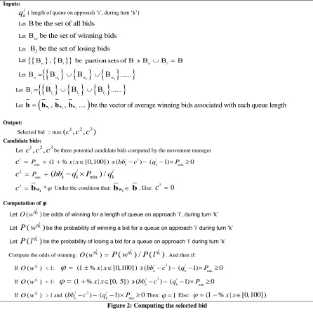
As Figure 2 indicates, movement managers compute three candidate bids and select the

Inputs:

i

k

q ( length of queue on approach ‘i’, during turn ‘k’)

Let be the set of all bids

Let _wbe the set of winning bids

Let _lbe the set of losing bids

Let    _w , _l be partion sets of      _{w l}

Let



   

 



1 2 3

...

w w  w  w

    

Let



   

 



1 2 3 ...

l l  l  l

    

Let b 





Output:

Selected bid = max( ,c c c1 2, 3) Candidate bids:

Let c c c1, 2, 3be three potential candidate bids computed by the movement manager

1 1

min (1 % | [0,100] ) ( ) ( 1) min 0

i i

k k

P x x bb c q P

c          

c2  P_min (bb_ki  q_ki P_min) /q_ki c3  bwi * Under the condition that: bwib. Else:

3

0

c 

Computation of φ

Let ( )

i k

q

O w be odds of winning for a length of queue on approach ‘i’, during turn ‘k’ Let ( )

i k

q

P w be the probability of winning a bid for a queue on approach ‘i’ during turn ‘k’

Let ( ) i k

q

P l be the probability of losing a bid for a queue on approach ‘i’ during turn ‘k’

Compute the odds of winning: _{O w}( qik)  _{P w}( qki) /_{P l}( qik)_{. And then if:}

If ( )

i k

q

O w < 1:   (1% |x x[0,100] )(bb_kic3)(q_ki  1) P_min0

If ( )

i k

q

O w = 1: (1 % | [0, 5] ) ( i 3) ( i 1) _min 0

k k

x x bb c q P

        

If ( )

i k

q

O w > 1 and ( i 3) ( i 1) _min 0

k k

bb c  q  P  Then:  1 Else: (1% |x x[0,100] )

Figure 2: Computing the selected bid

The first candidate bid is the highest possible amount (x% above nominal fee) that the

manager can bid, given a constraint that at least a nominal fee can still be paid to discharge

each of the remaining vehicles in queue. The second candidate is the highest bid possible if

the current funds are equally distributed among all drivers in queue. The third candidate bid

is the average winning bid for this queue length, adjusted downward if necessary to ensure

win/loss bids associated with the current queue ‘i’. The odds of winningO w( _i)are computed,

as well as the average winning bidbwiassociated with it (of course one can chose other

measures such as the median or 75th percentile bid as possible candidates instead of the

average bid). If necessary, this bid is adjusted to ensure that the movement manager remains

solvent. The details of this process can be found in Figure 2.

4.1.2. Drivers

Drivers make payments to the movement managers: first a fixed fee, and then voluntary

contributions. They learn about how much to pay as their short time in the game unfolds.

They have information about their queue position, and the win/loss record of their movement

manager from the time they join the queue. They make contribution decisions based on the

movement manager’s performance, their value of time, and the delay they have incurred.

Since drivers are transient players, they learn all this while in queue. Drivers do not pass on

their knowledge to other drivers.

A driver’s main objective is to transit the intersection in minimum time. When drivers arrive

at a given intersection, they have a desired delaydˆ_j. The value of the desired delay is a

function of their initial perception on movement manager’s ability to submit a winning bid;

the parameter ρj captures this aspect of their behavior. If driver j has an initial position of x0j

in the queue, and h_s is the saturation headway, then ˆ 0

j

j j s

d  x  h . If ρj = 1, then the drivers perspective is that the movement manager submits a winning bid every bidding cycle. On the

other hand, if ρj = 2.0, the assumption is that the movement manager submits a winning bid

every other bidding cycle. Therefore in this sense, the desired delay drivers want to achieve

influences the monetary contributions that they make voluntarily (please read rest of this

section to see why this is true). The value of ρj was set to 2.0 in the model realization used here.

Drivers constantly estimate the delay they anticipate incurring, k

j

k j

d to that reflects the movement manager’s win ratio and their position in queue. They

upward adjust the estimate if the movement manager loses (more likely to lose in the future),

and downward adjust it if the movement manager wins (increased chances of winning). The

estimate of k1

j

d  is computed using the following formula:

1 1

(1 ( ) / )

k k k

j j j

k k

j j s

d  d x   p  l D h (1) Where:

1

'( 1) '

estimated delayof vehicle'j'in queuein bidding cycle

k th

j

d   k

actual delay of vehicle ' 'in queue at the end of ' ' bidding cycle

k th

j

d  j k

position of vehicle ' 'in queue at the end of ' 'bidding cycle

k th

j

x  j k

1

( ) / probability that the movement manager loses in 'k+1 ' turn

k k th

j j

p  l D 

Drivers compute pk1( )l based on bidding outcome data since the time they joined until the end of the kth turn ( k

j

D ). The update procedure described in equation (1) is a modeling

decision created by the author. The idea is that as 1

( ) 1

k j

p  l  the estimate of anticipated

delay increases, and as pk_j1( )l 0the estimate of k1

j

d  goes down. Subsequent material

presented in this section provides more details on probabilistic reasoning used by the drivers.

Here the fundamental uncertainty lies in driver perceptions about movement manager’s

ability to submit a winning bid. The drivers take different actions (voluntary monetary

contributions, updating estimate of anticipated delay) after they update their perceptions of

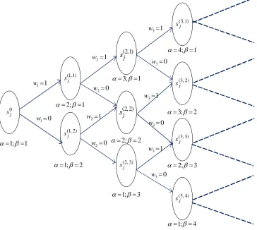
the movement manager’s performance. Drivers use Bayesian inference to update their belief about movement manager’s ability to submit a winning bid. Figure 3 presents schematic of

driver j’s decision network.

Every bidding cycle, the movement manager either submits a winning bid (outcome = W) or

P(L) = 1is the probability that the movement manager will lose. Here the distribution of



1 1

| ( , ) ~ ( , )

(1 )

( \ , )

( , )

Beta

P

 

    

 

  

  

 



 (2)

Since arriving drivers do not have any historical knowledge regarding their movement

manager’s ability to submit a winning bid, they assign equal probabilities to the movement

manager’s success/failure in the next bid event; this is achieved by setting 1;1.in equation (2). 0

j

s in the Figure 3 represents the state when driver j, joins the queue.

Let w_idenote the outcome of ith bidding cycle:

1

0 i

if the outcome is W w

if the outcome is L

_

 (3)

It is clear from Figure 3, that there will be (n+1) states at the end of nth bidding cycle and it is easy to see the update procedure for computing posterior probability. Suppose a driver

waiting in queue observes n successive bidding cycles. Among these, k outcomes were winning bids and (n-k) outcomes were losing bids. The posterior distribution is then given by:

1 1

| ~ ( , )

( | ) k (1 ) n k

n j

n j

D Beta k n k

P D  

  

       

  

  (4)

Drivers use this new information from the current bidding cycle to update their assessment of

whether their movement manager will win or lose subsequent bids. They compute

( \ n_j )

P H D

(Here ‘H’ is the hypothesis that the movement manger submits a winning bid) and P(H|Dn_j) using equation (2), and compute Bayes factor (which is the ratio of posterior odds to prior

( | ) ( | ) ( ) ( | ) n n j j n j

O H D P D H

O H P D H

K

  (5)

The left-hand side of equation (5) is the ratio of the posterior and prior odds, whereas the

right-hand side is the likelihood ratio, also known as ‘Bayes factor’, K. For the model presented here, K is the win to loss ratio at the end of a given bidding cycle. If K > 1, then

n j

D is more likely under H than underH, if K = 1, then n j

D is equally likely under either

hypothesis, and if K < 1, then n j

D is more likely under H than under H.

0 j s 1; 1   (1,1) j s (2,1) j s (1, 2) j s (2, 2) j s (2, 3) j s 1 1 w 2 1 w  2 0 w  1 0 w 2 0 w  2; 1   3; 1   2; 2   4; 1   1; 3   1; 2   2 1 w  (3,1) j s 3 1 w  3 0 w  3; 2   3 1 w  2; 3   3 0 w  3 1 w  1; 4   3 0 w  (3, 2) j s (3, 3) j s (3, 4) j s

Figure 3: Schematic of driver j’s decision network

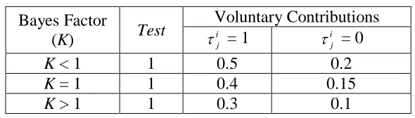
In every bidding cycle, the driver decides whether to make a voluntarily contribution. Table 1

shows the logic and the possible contributions.

Table 1: Table of possible voluntary contributions

Bayes Factor

(K) Test

Voluntary Contributions

i j

 = 1 i

j

 = 0

K < 1 1 0.5 0.2

K = 1 1 0.4 0.15

K > 1 1 0.3 0.1

The driver first determines the K as described previously. Then, the outcome of Test is determined. The variable Test equals 1 if k

j

d >dˆ_j, and it equals 0 if dk_j≤dˆ_j. Depending on the

values of K and Test, various possible contribution amounts pertain. For example, if K > 1,

Test = 1, and the driver has a high VOT, then the amount is 0.50. If the driver’s VOT is low, then it is 0.20. (The numerical values of the voluntary contributions have been chosen by the

author for illustrative purposes. They are logical, but not based on any empirical data.)

Then, there is a probability that the driver will actually make the contribution indicated in

Table 1. That probability is determined by the function shown in equation (6).

10 (( /( 1) 0.5)

( ) 1/ (1 K K )

p cont  e    (6)

To illustrate, if K is 1.0, i.e., the movement manager is as likely to win as to lose, then

p(cont) = 0.5. In other words, the probability that the driver will make a contribution is 50%.

As K → 0, i.e., the movement manager becomes very unlikely to win, and p(cont) → 1: the

4.1.3. Municipality

As mentioned earlier, rules govern how the game is played. The municipality defines these

rules and makes decisions about how to assign control among the movement managers. The

municipality also controls the times associated with green, yellow, and all-red durations, as

well as pauses in the bidding process. The municipality acquires information on queue

lengths for each approach from their respective movement managers. On the basis of this

information, the municipality tells the movement managers when to submit bids.

As the reader might imagine, the municipality is interested in an equitable and efficient

allocation of the intersection’s processing capacity. The municipality uses the bidding

process to allocate intersection capacity to different managers at different points in time.

These allocations are manifest in phase sequences and switching times. Furthermore, the

delays experienced by drivers are determined by the switching times, and there are costs

associated with those delays. The municipality can take these costs into consideration when

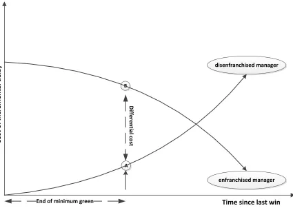
making decisions concerning switching times. The term for describing costs is ‘Marginal cost of incremental delay (MCID)’.

The following discussion helps describe these ideas further. Letg_min and c be the durations

of the minimum green and clearance interval respectively, and let be the cost of delay. It is

useful to recall that at the end of minimum green (g_min), both managers resubmit bids for

intersection control, if necessary. If the enfranchised manager loses, then the next earliest

time that manager is able to compete for intersection control is g_min 2c, so each vehicle on that manager’s approach incurs an additional delay equivalent tog_min 2c . On the other hand, if the disenfranchised manager loses the bid, then the next earliest time that manager

can compete for the intersection control is equal tog_ext, so each vehicle on that manager’s

System Incremental Delay (SID), and 2) Subject Approach Incremental Delay (SAID). It is

important to recognize that each method views the associated cost of delay differently.

Figure 4: Schematic showing cost of incremental delay

System Incremental Delay (SID): Equation (12) shows how to compute the SID-based cost.

It is the difference between delays that would be experienced by drivers on the enfranchised

versus disenfranchised approaches. This difference is multiplied by the cost of delay.

(

)

SID enf enf dis dis del

C  Q





c

Subject Approach Incremental Delay (SAID) – 2: Equation (13) shows how to compute the

SAID-based cost. It is the delay that would be experienced by drivers on the enfranchised

movement manager’s approach, multiplied by the cost of delay.

End of minimum green

C

o

st

o

f

in

cr

e

m

e

n

ta

l d

e

la

y

Time since last win

D

iff

e

re

n

tia

l c

o

st

disenfranchised manager

enfranchised manager

SAID enf enf del

C  Q  d 

c

Where,

SID

C  _{Marginal cost of system incremental delay}

SAID

C



enf

Q



enf

d  _{Future delay that would be experienced by drivers on the enfranchised}

Manager’s approach due to a shift in control

dis

Q



dis

d



manager’s approach

del

c



Based on one of these two these evaluations, the municipality adds an increment to the

minimum bid the disenfranchised manager has to submit to be assigned intersection control.

In the current realization, that minimum bid is the sum of the MCID (which is either CSIDor

SAID

C ) and the bid submitted by enfranchised manager.

min enf

bid  MCID  bid ₍₁₄₎

If the disenfranchised manager submits a bid higher thanbid_min, then that manager is assigned

control; otherwise control continues with the enfranchised manager.

Below are the rules by which the current realization of the game is played.

1) Movement managers collect an initial fee from the drivers; any additional monetary

contributions from the drivers are voluntary.

2) Assignment of intersection control is determined at the end of each discharge

headway (if vehicles are discharging), or at the end of a gap period if no subsequent

3) Assignment of intersection control pauses during discharge headways, minimum gaps

(if no subsequent vehicle arrives), clearance intervals, and minimum greens

(effectively for the duration of the clearance interval and the minimum green).

4) There are no maximum greens.

5) If only one movement manager has a queue, then control is assigned to that manager.

The lead vehicle in queue is discharged and the manager pays the municipality a

nominal fee.

6) If more than one movement manager has a non-zero queue, then assignment of

control is resolved through the submission of bids.

7) When bids are submitted, the process followed is single-stage, first-price sealed

bidding. That is, both movement managers submit bids. The winner is assigned

control, becomes the enfranchised manager, discharges the lead vehicle in queue, and

pays the municipality an amount equal to the bid submitted (i.e., the winning bid).

8) If the winner is already the enfranchised manager, bids pause for the minimum of the

discharge headway (if another vehicle arrives) or the gap time. If the winner is the

disenfranchised manager, then the duration of the pause is the change interval plus the

minimum green.

9) The municipality can elect to consider the marginal cost of incremental delays

(MCID) to make decisions about the assignment of intersection control.

10)If MCIDs are considered, the municipality can set a minimum for the bid (bid_min),

which the disenfranchised manager has to submit to take control of the intersection.

11)If the disenfranchised manager submits a bid higher thanbid_min, then control is

assigned to that manager. Otherwise, control continues to be assigned to the

enfranchised manager.

4.2.

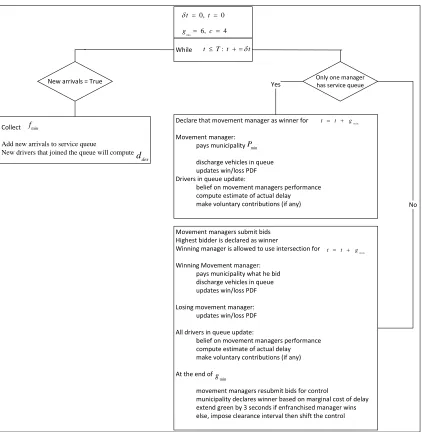
Flowchart for the Game Logic

The turn-by-turn pseudo code for the model logic is presented in Figure 4. The initial

step is 0.1 seconds and bidding events take place either at the end of vehicle discharge

headway or at the end of 3 seconds, whichever occurs first. What transpires during the

bidding event depends upon whether there are vehicles waiting to be serviced on both

approaches, just one approach or neither approach. Bidding is suspended during the change

interval and during the minimum green.

To incorporate clearance intervals, minimum greens and gaps, the following actions are

taken. For the clearance intervals and minimum greens, if control shifts from one manager to

another as a result of the bidding process, bid submission ceases for a clearance interval plus

a minimum green. At the end of this time period, managers with non-zero queues again

submit bids for use of the intersection space. For the gaps, bidding is suspended until the end

of the gap time or the next vehicle arrival, whichever occurs first.

During the bidding event, if only one movement manager has a service queue that manager is

an automatic winner; he is allowed to use the intersection space for a duration equivalent to

the minimum green (if control shifts) or the minimum of the 3-second gap or the headway to

the next arriving vehicle. For every vehicle discharged in this manner, the manager pays a

nominal fee to the municipality.

If both movement managers have service queues, then both movement managers submit bids

(refer to the previous section for details about how the bids are computed); the winning

bidder is selected by the municipality, and the winner is allowed to use the intersection space

for the same duration described earlier; the winning movement manager pays the

municipality what was bid (first-price bidding); and discharges the first-in-queue vehicle at

saturation headway. All movement managers then update their win/loss PDFs using the

results of the bid. Remaining drivers update their belief about their movement manager’s

likelihood of winning, they re-compute their k j

d , and decide whether or not they want to