High-Resolution Crossover Maps for Each Bivalent of
Zea mays
Using
Recombination Nodules
Lorinda K. Anderson,*
,1Gregory G. Doyle,
†Brian Brigham,* Jenna Carter,* Kristina D. Hooker,*
Ann Lai,* Mindy Rice* and Stephen M. Stack*
*Department of Biology, Colorado State University, Fort Collins, Colorado 80523 and †Department of Agronomy, University of Missouri, Columbia, Missouri 65211
Manuscript received April 11, 2003 Accepted for publication June 17, 2003
ABSTRACT
Recombination nodules (RNs) are closely correlated with crossing over, and, because they are observed by electron microscopy of synaptonemal complexes (SCs) in extended pachytene chromosomes, RNs provide the highest-resolution cytological marker currently available for defining the frequency and distri-bution of crossovers along the length of chromosomes. Using the maize inbred line KYS, we prepared an SC karyotype in which each SC was identified by relative length and arm ratio and related to the proper linkage group using inversion heterozygotes. We mapped 4267 RNs on 2080 identified SCs to produce high-resolution maps of RN frequency and distribution on each bivalent. RN frequencies are closely correlated with both chiasma frequencies and SC length. The total length of the RN recombination map is about twofold shorter than that of most maize linkage maps, but there is good correspondence between the relative lengths of the different maps when individual bivalents are considered. Each bivalent has a unique distribution of crossing over, but all bivalents share a high frequency of distal RNs and a severe reduction of RNs at and near kinetochores. The frequency of RNs at knobs is either similar to or higher than the average frequency of RNs along the SCs. These RN maps represent an independent measure of crossing over along maize bivalents.
M
AIZE (Zea maysL.) is one of the first model organ- ern1967;de la Torreet al.1986;Jones1987;Shermanisms in which the power of genetics was produc- andStack1995).
tively merged with cytology to create the new field of One way to relate linkage maps to the structure of cytogenetics (reviewed by Rhoades 1984). The ability chromosomes is to observe the location and frequency to recognize all 10 maize chromosomes in pachytene of crossing over along chromosomes by means other squash preparations was key for relating each chromo- than linkage analysis. To a degree this has been accom-some to a specific linkage group (McClintock 1931, plished in squash preparations by observing the number 1933;RhoadesandMcClintock1935). Subsequently, and positions of chiasmata on late diplotene-diakinesis maize chromosome cytology has remained a fertile field bivalents (Jones1987). Unfortunately, for most species, for investigation (e.g.,Daweet al. 1994;Freelingand including maize, this is a relatively inaccurate,
low-reso-Walbot1994;Basset al.2000;Muehlbaueret al.2000; lution method because (1) twists can be mistaken for
SadderandWeber2002) that has been accompanied chiasmata, (2) nearby chiasmata may not be resolved, by the development of sophisticated maize linkage maps (3) chromosomes are comparatively short when chias-(e.g.,Daviset al.1999;Sharopovaet al.2002). However, mata are visible, and (4) it is difficult to relate most integration of linkage maps with chromosome structure bivalents to specific pairs of chromosomes (Stacket al. has been difficult in maize (as well as in other organisms) 1989;ShermanandStack1995;Stevensonet al.1998). because crossing over is not evenly distributed along Another method for cytologically assessing crossing over the length of chromosomes. For example, crossing over has been developed recently using fluorescent antibod-is typically uncommon in heterochromatin and centro- ies to label MLH1p, a mismatch repair protein that is meres compared to euchromatin (e.g.,Mather 1939; present at crossover sites during pachytene (Baker et for reviews seeComings1972;Resnick1987), and even al. 1996; Hunter and Borts 1997; Anderson et al. in euchromatin, where the bulk of crossing over occurs, 1999;Moenset al.2002). Because MLH1 signals appear the frequency of crossing over can vary considerably as discrete fluorescent foci on pachytene bivalents that from one part of a chromosome to another (e.g.,South- are 5–10 times longer than bivalents at diakinesis, MLH1
foci can be mapped at higher resolution than chiasmata can. However, the application of this technique to map-1Corresponding author:Department of Biology, Colorado State
Uni-ping crossovers has been limited to birds and mammals
versity, Fort Collins, CO 80523.
E-mail: [email protected] so far (e.g.,Pigozzi2001;Froenickeet al.2002),
grown in a temperature-controlled greenhouse with
supple-haps because the antibodies were raised to mammalian
mental lighting. All inversion heterozygotes were in KYS
back-MLH1 proteins, and these antibodies do not bind to
ground.
their plant counterparts (our observations). While rep- Diakinesis chromosome squashes:Anthers containing diaki-resenting a significant improvement over chiasmata to nesis-stage cells were fixed for 1–24 hr in 1:3 acetic ethanol. map crossover events, analysis of MLH1 fluorescent foci After clearing the anthers for 1–5 min in 45% acetic acid, the meiotic cells were squeezed out of the anthers in a fresh drop
is still limited by the resolution of the light microscope.
of 45% acetic acid and squashed lightly under a siliconized cover
The highest-resolution method available to map the
glass. The cover glass was removed using dry ice, the slide was
frequency and location of crossover events cytologically
allowed to air dry, and chromosomes were stained with 2%
remains analysis of late recombination nodules (RNs; aceto-orcein under a cover glass with brief heating over an sometimes abbreviated as LNs) on synaptonemal com- alcohol lamp. After staining, cover glasses were removed by plexes (SCs;e.g.,Carpenter1975; reviewed byZickler inverting the slide over 95% ethanol. Before the preparations dried, new cover glasses were mounted with Euparal.
Com-andKleckner1999;AndersonandStack2002). RNs
plete sets in which all chromosomes were separate and
inter-are proteinaceous ellipsoids,ⵑ100 nm in their longest
pretable were photographed using a⫻100 PlanApo objective
dimension, which lie on SCs (that is, pachytene
biva-and a digital camera attached to an Olympus Provis light
lents). RNs are closely correlated with crossovers and microscope.
lie at sites where chiasmata will form later (Carpenter Pachytene SC spreads:SC spreads were prepared on
plastic-coated slides as described byStackand Anderson(2002).
1975, 1979; von Wettstein et al. 1984;Marcon and
SC spreads were stained with 2% uranyl acetate followed by
Moens 2003). The proposed role of RNs as molecular
Reynold’s lead citrate (UP) or with 33% silver nitrate
(Sher-factories for crossing over has been corroborated
re-man et al.1992). The slides were scanned using phase light
cently by work showing that the MLH1 protein is a microscopy, and good SC spreads on plastic were picked up component of late RNs (Moens et al.2002). The high onto 50- or 75-mesh grids. The grids were examined in an AEI resolution of RN analysis is due not only to the observa- 801 electron microscope, and SC spreads without detectable stretching and with kinetochores were photographed at a
mag-tion of RNs on relatively long pachytene chromosomes,
nification of⫻1600 or⫻2500. In total, 2080 individual SCs
but also to the small size of RNs compared to chiasmata
from 290 sets were identified and mapped with regard to RNs.
(0.1mvs.1m, respectively) and to the use of electron
Both total RN number and total SC set length (the combined
microscopy to resolve RNs. length of all SCs in a cell) could be assessed for 206 of these
The most useful cytological maps of crossing over are SC sets. In the remainder of the sets, certain of the SCs could those in which every bivalent can be identified unequivo- not be identified, usually due to unclear or missing kineto-chores. Some SCs had a small amount of asynapsis, particularly
cally and related to a specific linkage group. This has
near the ends, and may have been in the very earliest stages
not been possible in many organisms, and, in lieu of
of diplotene.
this, some studies have pooled crossover data from
chro-Measurements:Electron microscope negatives were scanned
mosomes of similar size and arm ratios (Southern into a computer using a Hewlett-Packard ScanJet 4c and Adobe
1967; Anderson et al. 1999). In other studies, it was Photoshop (version 5.0) software. Montages of SC spreads
were assembled using Adobe Photoshop. Proper tracing of
possible to identify some of the bivalents using either
each SC and the position of kinetochores and RNs were
deter-a combindeter-ation of reldeter-ative lengths deter-and deter-arm rdeter-atios (e.g.,
mined directly from the negatives using a⫻8 magnifying loupe
LaurieandJones1981;Pigozzi2001) or fluorescence
and recorded onto prints of the montages. One lateral ele-in situhybridization of chromosome-specific sequences ment from each SC was measured in micrometers using the (Lynnet al.2002;Teaseet al.2002). Thus far, only two computer program MicroMeasure (Reeves 2001). Total SC studies have mapped crossing over on every bivalent in length varied from set to set, but the relative length of SCs and SC arms,i.e., arm ratios, within each set remained
consis-a set, one using RNs on tomconsis-ato SCs thconsis-at were identified
tent. SCs were identified by relative lengths (percentages of
by relative lengths, arm ratios, and patterns of
hetero-total SC length for the set) and arm ratios (length of the long
chromatin (ShermanandStack1995) and the other
arm divided by length of the short arm). RNs were recognized
using MLH1 foci on mouse autosomal SCs after chromo- using criteria of size, shape, staining intensity, and association some-specific painting (Froenicke et al. 2002). Here with SC as described by Stack and Anderson (2002). RN we report such an analysis in maize. For this, we first positions were measured and expressed as a percentage of the arm length from the centromere. Using average lengths
prepared an SC karyotype on the basis of relative lengths
for each of the 10 SCs and their average arm ratios, each of
and arm ratios for the maize inbred line Kansas Yellow
the SCs was divided into 0.2-m segments, and each observed
Saline (KYS). Each SC was identified and related to a
RN was placed into one of these segments on the basis of its
specific maize chromosome and linkage group. Most SC original relative position from the centromere. For those SCs identifications were verified using inversion heterozygotes. in which an arm was not divisible by two, the most proximal interval was made 0.3m rather than 0.2m. After compiling
We then determined the frequency and distribution of
the RN data, the genetic map length of each SC was calculated
RNs (crossing over) on each of the 10 maize SCs.
by determining the average number of RNs per SC and then multiplying by 50 (one RN⫽one crossover⫽50 cM).
Statistics:The program Minitab (version 13) was used for MATERIALS AND METHODS
statistical analyses and for preparing histograms. The smooth-ing (Lowess) lines were based on the histograms (Minitab Plants:Maize inbred KYS and heterozygotes for inversions
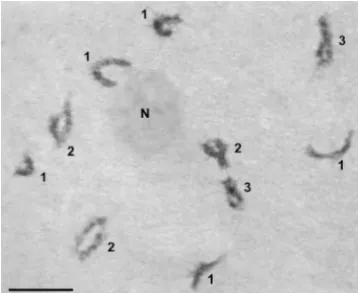
Figure 1.—Complete set of silver-stained spread SCs from maize KYS. Each SC has been identified by its relative length and arm ra-tio and numbered accord-ingly. Arrows indicate the location of RNs. The two RNs on the short arm of SC 6 are so close together that they would likely result in a structure that would be in-terpreted as a single chi-asma during diakinesis. Lat-eral element thickenings can be observed on several SCs (e.g., 1S, 2S, 7S, 10L). Such thickenings are more commonly observed with sil-ver staining than with ura-nyl acetate-lead citrate stain-ing. K, kinetochore; S, short arm; L, long arm. Bar, 5m.
RESULTS in relative length between 2 (or sometimes 3) SCs was
minimal, but the arm ratios were noticeably different. SC karyotype:SC spreads were prepared by exposing
The average relative length and average arm ratio for protoplasts to a hypotonic solution containing a small
each ranked SC from the 30 sets are presented in Table amount of nonionic detergent (StackandAnderson
1 along with the same information for five other karyo-2002). During this procedure, the cytoplasm as well as
types produced from squashes, three-dimensional re-the chromatin surrounding each SC decondenses to
constructions, and SC spreads. Except for absolute total become almost invisible, while SCs and RNs are
rela-lengths of complete sets and the arm ratio of SC 6 tively unaffected (Figure 1). Dispersion of the
chroma-that carries the NOR, the similarity of the karyotypes is tin means that such features as chromomeres and knobs
striking. Overall, the SCs decrease gradually in average are not visible to help identify SCs. In addition, the
relative length from SC 1 (14.8%) to SC 10 (6.8%), but nucleolus is usually dispersed in these preparations, so
the length positions of SC 4 and SC 5 have been reversed it is not possible to detect the association of the
nucleo-to reflect the standard pachytene chromosome karyo-lus with the nucleokaryo-lus organizer (NOR) on the short
type. With regard to arm ratios, each ranked SC group arm of SC 6 (McClintock1934). This means that SC
is statistically different from the SC group immediately identification must rely on relative length and arm ratio.
preceding or succeeding it (P⬍0.002, two-samplet-test). Arm ratios can be determined only when kinetochores
Thus, each SC in a set can be identified accurately on are visible in SC spreads that are probably in mid- to
the basis of its relative length and arm ratio. late pachytene.
To verify that our SC identifications were consistent To prepare the karyotype, SC spreads were selected
with the genetic linkage groups, we analyzed spreads of using the following criteria: (1) each of the 10 SCs could
SCs from plants that were heterozygous for one of the be followed along its entire length, (2) the kinetochore
following inversions:1d,2i, 3c,4c, 5d, 6b, 7a, 8c, 9b, or was visible on each SC, and (3) SCs were not visibly
10a(Figure 2;Doyle 1994). Unfortunately, obtaining stretched. Thirty sets of SCs that met these criteria were
spreads that contained inversion loops along with distin-measured for lengths and arm ratios. Then SCs in each
guishable kinetochores on each SC proved to be diffi-set were ordered according to their relative lengths. If
cult. For example, no SC spreads from the inversion necessary, the order of an SC was changed so that the
heterozygotesIn8candIn10afulfilled these two criteria, arm ratios for each SC were consistent with pachytene
and only 27 SC sets (In1d⫽2;In2i⫽6;In3c⫽3;In4c⫽4; maps (Table 1). Out of the (10⫻30⫽) 300 SC length
In5d⫽ 2;In6b ⫽1;In7a⫽ 5;In9b ⫽4) for the other positions, 55 (18%) were changed on the basis of the
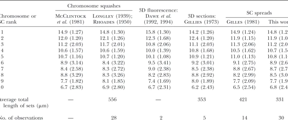
TABLE 1
Comparison of selected karyotypes for maize
Chromosome squashes
SC spreads 3D fluorescence:
Chromosome or McClintock Longley(1939); Daweet al. 3D sections:
SC rank et al.(1981) Rhoades (1950) (1992, 1994) Gillies(1973) Gilles(1981) This work
1 14.9 (1.27) 14.8 (1.30) 15.8 (1.30) 14.2 (1.26) 14.9 (1.24) 14.8 (1.27)
2 12.0 (1.20) 12.1 (1.26) 12.3 (1.68) 12.4 (1.20) 11.9 (1.15) 11.9 (1.08)
3 11.2 (2.03) 11.7 (2.01) 10.8 (2.06) 11.1 (2.03) 11.3 (2.06) 11.2 (2.02)
4 10.6 (1.57) 10.6 (1.59) 10.0 (1.39) 10.8 (1.68) 10.5 (1.62) 10.7 (1.56)
5 10.7 (1.16) 10.7 (1.20) 10.1 (1.08) 10.9 (1.21) 11.0 (1.13) 10.8 (1.10)
6 8.9 (3.14) 8.4 (3.22) 9.5 (3.41) 9.2 (3.01) 9.1 (2.75) 8.9 (2.63)
7 8.4 (2.58) 8.3 (2.72) 9.0 (2.38) 8.5 (2.38) 8.8 (2.67) 8.7 (2.76)
8 8.8 (3.29) 8.3 (3.26) 8.2 (2.83) 8.8 (2.92) 8.2 (2.99) 8.5 (3.04)
9 7.7 (1.82) 8.1 (1.85) 7.4 (1.69) 8.0 (1.89) 7.7 (2.09) 7.7 (1.92)
10 6.7 (2.83) 6.9 (2.80) 6.7 (2.31) 6.2 (2.43) 6.5 (2.54) 6.8 (2.43)
Average total — 556 — 353 421 331
length of sets (m)
No. of observations — 28 2 5 14 30
The karyotypes were prepared using a variety of techniques including light microscopy of pachytene chromosome squashes, deconvolution-based, three-dimensional fluorescence light microscopy of intact pachytene nuclei, three-dimensional electron microscopic reconstructions of pachytene nuclei from serial thin sections, or electron microscopy of SC spreads. In all cases, primary microsporocytes from maize inbred KYS were used. For each karyotype, the average relative length of each SC is presented first as a percentage of the total length of the SC set, followed by the average arm ratio in parentheses.
identifications (Figure 2). Because an inversion loop even if not all of the SCs could be individually identified (usually because of the absence of discernible kineto-with associated asynapsis on its borders can alter the
expected relative length and arm ratio for the inversion chores). These complete sets of SCs averaged 20.7 RNs per SC set, a difference of ⬍1% when compared to loop SC, the nine normal chromosomes in a set were
identified using relative lengths and arm ratios, with using RN averages for individual SCs. Thus, using RNs, we estimate that the total map length for maize inbred the “missing” SC being identified as the SC with the
inversion loop. For each of the eight inversion heterozy- KYS is between (20.5 RNs ⫻ 50 cM/RN ⫽) 1025 cM and (20.7 RNs⫻50 cM/RN⫽) 1035 cM.
gotes in which this test was possible, the identification
of the inversion loop SC corresponded with the appro- Chiasma frequency per cell: To compare rates of crossing over in KYS maize determined from RNs to priate chromosome. This result confirms that our SC
iden-tifications are consistent with established linkage groups. those determined from chiasmata, we analyzed at least 50 squashes of chromosome sets at diakinesis from each We examined 290 sets of SCs with RNs and were able
to identify 2080 (ⵑ72%) individual SCs (Table 2, Figure of 5 plants (Figure 4) and at least 10 SC spreads from each of 10 plants (Table 3). No single plant was analyzed 3). Some SCs were easier to identify than others, so
the number of each SC analyzed for RNs varies. For for both chiasmata and RNs. Each plant, regardless of the method of analysis, demonstrated large cell-to-cell example, SC 2, a long SC with an arm ratio near 1.0,
and SC 10, the shortest SC, were relatively easy to iden- variability (up to twofold) in the number of crossovers observed. While there were no significant differences tify, and as a result, we made 247 observations of each.
In contrast, the number of observations for SC 6 and among plants in variance for chiasmata or for RNs (Bart-lett’s test and Levene’s test,P⬎0.2), there were signifi-SC 7 was lower (n⫽176 and 178, respectively) because
they are similar in both relative length and arm ratio cant differences among plants in the mean number of crossovers per cell on the basis of both chiasmata and more difficult to distinguish from one another.
Nevertheless, these data represent the highest number (ANOVA; P ⬍ 0.001) and RNs (ANOVA; P ⬍ 0.001). Because the plants were all from the same inbred strain of observations of RNs on individual SCs made for any
organism except tomato (ShermanandStack1995). and presumably had the same genetic makeup, we ex-plored the possibility that environmental conditions RN frequency per cell: On the basis of the average
frequency of RNs per SC, there is an average of 20.5 were responsible for the differences in mean crossover frequency. The plants analyzed for chiasmata were all RNs per cell (Table 2). To verify that this number is
used. Bivalents with two crossovers were observed more often for chiasmata than for RNs, while bivalents with three or more crossovers were observed more often for RNs than for chiasmata. The difference in resolution of the two techniques may contribute to these observed discrepancies.
Relationship between RN frequency and SC length: For 206 SC sets, we were able to determine both total RN number and total SC set length (although not all SCs could be identified in each spread; Figure 5A). The slope of the regression is significantly different from zero [total RNs⫽(0.026⫻total SC length)⫹11.8,P⬍ 0.001,r2⫽16.3%]. Thus, SC set length and RN number
per set are positively related, withⵑ16% of the variation in RN number explained by SC set length.
When the 10 maize bivalents are considered sepa-rately (n⫽2080 SCs, Tables 1 and 2), there is a strong positive relationship between average RN frequency and average SC length, with 96% of the variability in average RN frequency related to average SC length [Figure 5B; y⫽(0.042⫻SC length)⫹0.66,r2⫽96.2%]. A similar
relationship is observed when average SC arm lengths are compared to the average number of RNs per arm
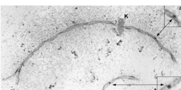
Figure2.—Complete SC spread stained with uranyl acetate- [Figure 5C,y⫽(0.044⫻SC length)⫹0.31,r2⫽96.5%]. lead citrate from a maize plant heterozygous forIn7a. Each
For both regressions, the slope andy-intercept are
sig-SC has been labeled at the kinetochore (K) with the
appro-nificantly different from zero (P⬍0.001). Thus, average
priate SC number on the basis of its relative length and arm
RN frequency is closely correlated with individual SC
ratio. The inversion loop in the long arm of SC 7 can be seen
in the lower left of the spread. Kinetochores from different length, whether one considers arm lengths separately
SCs are often fused (6K and 8K, 1K and 10K, 4K and 5K). or bivalent length as a whole. There are no obvious lateral element thickenings on any of
Distribution of RNs along SCs:Histograms showing
the SCs. Bar, 5m.
the distribution of RNs along each SC are presented in Figure 6. Each SC is represented by thex-axis with the short arm to the left and the kinetochore (kc) marked four years from 1998 to 2002, again using plants grown
in the same greenhouse. SC spreads from 8 of the 10 with a vertical line beneath the axis. Each SC is divided into 0.2-m segments with the number of RNs observed plants were prepared in the summer (April–September)
and SC spreads from 2 of the plants were prepared in in each segment represented by a vertical bar. Two lines are superimposed over each distribution. One is a the fall (October–March). The average number of RNs
per cell was 19.8 and 21.5 for the 2 winter-grown plants smoothing (Lowess) line derived from the data ( Cleve-land1979), which shows the general trend of crossing and 17.0–23.1 for the 8 summer-grown plants. Although
the data are limited, this pattern of RN numbers does over along each SC. The smoothing line minimizes varia-tion regardless of whether the variavaria-tion is caused by not support the hypothesis that environmental factors
are responsible for the differences in RN numbers ob- sampling errors or by localized differences in crossover frequency. The second superimposed line is horizontal served.
Because the ranges of values for chiasmata and for and represents the average number of RNs observed per 0.2-m interval for each SC. Intervals that differ RNs were similar among plants (even though there were
significant differences in mean crossover frequency considerably from the horizontal lines represent hot (above average) or cold (below average) regions for among plants), the data for chiasmata and RNs were
pooled separately and compared. The average number crossing over.
All of the SCs share the general characteristics of a of RNs per cell wasⵑ10% higher (20.6) than the average
number of chiasmata (18.9; Table 3). In addition to high frequency of RNs in distal regions (including the very ends of SCs) and a low frequency of RNs in proximal determining the average number of crossovers per cell,
we also examined the frequencies of bivalents with 0, regions, i.e., around kinetochores (Figures 6 and 7). The distributions of RNs on SCs 2, 4, and 9 indicate 1, 2, and 3 or more RNs and chiasmata (Table 3). The
frequencies of bivalents with zero and one crossover per that a few RNs occur within kinetochores. This is an artifact due to compiling data from SCs that vary some-cell were the same whether RNs or chiasmata were used.
TABLE 2
Predicted map length based on the average number of RNs per SC compared to classical genetic and molecular (IBM) linkage maps
SC Genetic mapa,b IBM mapa,c
No. of SCs Average Equivalent Equivalent Equivalent
SC no. observed no. of RN cMd cM RNe cMf RNe
1 216 2.69 134.3 258 5.2 325.3 6.5
2 247 2.37 118.4 224 4.5 204.2 4.1
3 189 2.22 110.9 216 4.3 228.4 4.6
4 196 2.14 107.1 172 3.4 228.3 4.6
5 203 2.21 110.6 185 3.7 202.6 4.1
6 176 1.81 90.6 144 2.9 164.2 3.3
7 178 1.86 93.0 128 2.6 188.7 3.8
8 194 1.80 90.2 177 3.5 189.2 3.8
9 234 1.85 92.7 178 3.6 193.9 3.9
10 247 1.54 76.9 174 3.5 157.4 3.1
Total 2080 20.5 1024.7 1856 37.1 2082.2 41.8
aFrom http://www.agron.missouri.edu/cMapDB/cMap.html (March 2003). bGenetic map is the classical genetic map, compiled by Ed Coe from cooperators. cIBM is an intermated B73/Mo17 recombinant inbred high-resolution molecular map. dThe average number of RNs⫻50 cM/RN.
eCentimorgans divided by 50.
fThis molecular map includes recombination events from three meioses (K.Cone, personal communication),
so the centimorgans presented on the web site have been divided by 3 here for the purpose of comparison using the standard definition of centimorgans (Tamarin2002).
to the kinetochore, we did not observe any RNs that segments contain 48% (2061/4271) of all RNs observed while the most proximal segments contain 4% (156/ were clearly within kinetochores (Figure 7). In addition
to the general trends in the distribution of crossing over 4271) of all RNs observed. Thus, over the same SC length, distal regions have 12 times more crossing over that all SCs share, each SC also has a distinct pattern
of RNs along its length. than proximal regions do.
Maize KYS has five knobs, two on short arms (1S, 9S) To quantify the difference in RN frequency between
distal and proximal segments, we divided each SC arm and three on long arms (5L, 6L, 7L;Daweet al.1992;
Chenet al.2000). The location of each knob is indicated into five equal (20%) segments, pooled the total
num-ber of RNs observed for all of the most distal segments, by a horizontal line beneath the appropriate SC in Fig-ure 6. Overall, the frequency of RNs in knob regions is and pooled the total number of RNs for all proximal
segments. The combined distal segments for all SCs either about the same as the average for the SC as a whole (5L, 6L, 7L) or higher (1S, 9S). This is particularly represent (0.20⫻331m total SC length⫽) 66.2m
in length as do the combined proximal segments. If true for the knob on the tip of the short arm of SC 9, which has a frequency of RNs that is twice as high as RNs were distributed evenly along the length of all SCs,
then each 20% segment would haveⵑ20% of the total the average for SC 9 (7vs.3.4 RNs per 0.2-m interval). In contrast, the NOR region on the short arm of SC 6 number of RNs observed. Instead, the most-distal SC
different maize lines, aside from the observation that the number and location of heterochromatic knobs may vary (Longley1939;McClintocket al.1981;Dempsey
1994). However, while the presence of knobs can affect the length and arm ratios of mitotic chromosomes, the presence or absence of knobs has little effect on the relative length and arm ratios of SCs because hetero-chromatin is underrepresented in SC length (Stack
1984;Jonesandde Azkue1993). Thus, it is likely that the KYS SC karyotype applies in large measure to all maize lines.
Within animal and plant species (including maize) and even within individuals, there may be as much as a twofold variation in the absolute lengths of sets of
pachy-Figure4.—Diakinesis chromosome squash from maize KYS.
The counted number of chiasmata is indicated next to each tene chromosomes or SCs. However, the relative length
bivalent. With the exception of chromosome 6 that is associ- and arm ratio for each chromosome or SC in a set remains ated with the nucleolus (N), none of the chromosomes can
constant (Moses et al. 1977; Gillies 1981; Sherman
be identified. Bar, 10m.
andStack1992; our observations). This indicates that each chromosome/SC in a set responds in a propor-tional way to changes in the length of the entire set. has a slightly reduced level of RNs compared to the
Chromosome numbering in maize is based primarily average for SC 6 (1.6vs.2.2 RNs per 0.2-m interval),
on relative length with the longest chromosome num-but this lower level could be due to its proximity to the
bered 1, ranging down to the shortest numbered 10. kinetochore (Figure 6).
However, in each karyotype reported for maize, chro-mosome/SC 5 is slightly longer than chrochro-mosome/SC
DISCUSSION 4 (Table 1). This discontinuity in numbering arose
be-cause maize chromosomes were numbered initially us-SC identification: We have prepared a karyotype for
ing mitotic chromosomes that differ slightly in relative SCs from KYS maize on the basis of relative lengths and
length from pachytene chromosomes (McClintock
arm ratios (Figure 1; Table 1). This SC karyotype is very
1929;Rhoades1955;Carlson1988). In addition, chro-similar to other maize pachytene karyotypes that have
mosome/SC 8 is longer than chromosome/SC 7 in been prepared using a number of different techniques
some karyotypes but not in others (Table 1). These (aceto-carmine-stained pachytene chromosome squashes,
differences in relative length between different maize 4⬘,6-diamidino-2-phenyindole-stained intact pachytene
karyotypes are small and may represent either measure-nuclei, three-dimensional reconstructions of pachytene
ment error or natural variation within populations. In nuclei from serial thin sections, and SC spreads). The
either case, these chromosomes are still readily distin-inbred KYS line of maize generally has been used in
guished from each other on the basis of differences in these studies because KYS pachytene chromosomes
sep-their arm ratios. In addition, we were able to verify the arate well during squashing and spreading, making them
identity of SCs 1, 2, 3, 4, 5, 6, 7, and 9 using inversion easier to analyze than pachytene chromosomes from
heterozygotes. Although not verified by inversion het-many other maize lines (Dempsey 1994; our
unpub-erozygotes, our identification of SCs 8 and 10 is also lished observations). In any case, there is little difference
in the basic pachytene chromosome karyotype between firm because both SC 8 and SC 10 can be readily
distin-TABLE 3
Comparison of crossover frequency for maize KYS using chiasmata and RNs
No. of cells Mean no. of RNs No. of bivalents with 0–6 crossoversa
(bivalents) or chiasmata (SD)
observed and range 0 1 2 3 4–6
RNs 151 20.6 (3.3) 14 363 743 312 78
10 plants (1510) 13–33 (0.9) (24.0) (49.2) (20.7) (5.2)
Chiasmata 278 18.9 (2.5) 31 667 1673 402 7
5 plants (2780) 12–26 (1.1) (24.0) (60.2) (14.5) (0.3)
Pvaluesb ⬍0.001 0.56 0.97 ⬍0.001 ⬍0.001 ⬍0.001
aNumbers in parentheses represent percentages.
location of the NOR in spreads. However, we did not observe any unusual fragmentation or any detectable stretching of the SC in the short arm of maize SC 6. Whatever the cause of the differences in arm ratio for chromosome/SC 6, we are confident that we can iden-tify SC 6 because the arm ratio for SC 6 is consistent between sets of SC spreads, SC 6 can be separated reli-ably from the other SCs, and SC 6 has been verified to correspond to chromosome 6 by analysis of SC spreads from inversion heterozygotes forIn6b.
Estimating crossover frequency using different meth-ods:Some controversy surrounds estimates of crossover frequency that have been determined using chiasmata, RNs, and linkage maps (e.g.,Nilssonet al.1993; Sher-manandStack1995;Sybenga1996;Kinget al.2002a). Typically, saturated or nearly saturated classical linkage maps indicate higher crossover rates than chiasma counts, and molecular linkage maps often indicate even higher crossover rates (e.g.,Nilssonet al.1993;Moran
et al.2001;Kinget al.2002a; Table 3). This also appears to be the pattern in maize where chiasma counts range from an average of 17–21 per cell when diakinesis-meta-phase I chromosomes are used (Beadle 1933; Ayo-noaduandRees1968;Pagliariniet al.1986; Table 3) although higher averages (27–37 per cell) are possible when longer diplotene chromosomes are used (in which chiasmata are more difficult to distinguish from twists;
Beadle 1933; Darlington1934). In comparison, ge-netic and molecular linkage maps indicate 37 and 42 crossovers per cell, respectively (Table 2). This problem
Figure5.—Scatter plots and regressions for (A) total SC has been addressed recently byKinget al.(2002a), who
set length and total RN number (y⫽0.026x ⫹11.82,r2⫽
introgressed a single chromosome of Festuca pratensis 0.16), (B) average SC length and average RN frequency (y⫽ intoLolium perenneto create a monosomic substitution 0.042x ⫹ 0.66,r2⫽ 0.96), and (C) average SC arm length
line (hereafter referred to as the Festuca/Lolium
biva-and average RN frequency (y⫽0.044x⫹0.31,r2⫽0.97).
lent). TheF. pratensischromosome synapses and recom-bines with the homeologous L. perenne chromosome, although the two chromosomes can be distinguished guished from the other SCs and from each other on
the basis of their relative lengths and arm ratios. from one another using genomicin situhybridization.
King et al. (2002a) compared the recombination fre-The most striking difference among maize karyotypes
involves the arm ratio for chromosome/SC 6. The aver- quency for this homeologous bivalent using both ampli-fied fragment length polymorphism markers and chias-age arm ratio is 3.0 or higher for squashed pachytene
chromosomes and sectioned SCs, but only 2.6–2.7 for mata. They found a 1:1 relationship between crossovers detected by the two methods. They suggest that chiasma SC spreads (Table 1). Since the short arm of
chromo-some/SC 6 carries the NOR, it is likely that differences counts tend to somewhat underestimate the amount of crossing over due to difficulty in resolving nearby chias-between the karyotypes somehow involve the nucleolus.
Typically, a single large nucleolus is visible in primary mata, while molecular maps tend to inflate the amount of crossing over due to errors in typing and the use of microsporocytes that are fixed before squashing or
sec-tioning (Rhoades1950;Daweet al.1994). In contrast, different computer programs with different algorithms to generate the maps.Kinget al.(2002a) also pointed SC spreads are prepared by exposing live cells to a
hypo-tonic solution in which nucleoli and chromatin are dis- out that differences in map lengths are not surprising, given that various investigators employed a variety of persed before fixation. The larger arm ratio of SC 6 in
squashes compared to SC spreads could be due to rela- mapping techniques on different mapping populations. Recently,KnoxandEllis(2002) showed in pea (Pisum tive shortening of the NOR short arm in squashes
(per-haps because the nucleolus obscures part of the arm) sativum) that excess heterozygosity in the mapping pop-ulation can also lead to inflation of the molecular map or lengthening of the short arm in SC spreads. In this
Figure6.—Histograms showing the distribution of RNs along the length of each maize SC. Each SC is represented on the x-axis with the short arm to the left and the position of the kinetochore (kc) marked with a vertical line. The positions of the NOR (6S) and knobs (1S, 5L, 6L, 7L, 9S) are indicated as short horizontal bars beneath thex-axis. The histogram bars represent the total observed number of RNs in each 0.2-m SC length interval. Superimposed over each distribution is a thick smoothing line that shows the general trend of the RN distribution as well as a thinner horizontal line that represents the average number of RNs in each 0.2-m interval.
molecular markers and that chiasmata and RNs yield zero or one RN (Table 3). When higher categories of crossing over are compared, the number of bivalents good estimates of crossover frequency.
Here, we show that in KYS maize the frequency of chias- with two chiasmata is higher than the number of biva-lents with two RNs, while the number of bivabiva-lents with mata compares well with the frequency of RNs, particularly
Figure6.—Continued.
in resolution between RNs and chiasmata (Stacket al. Inbred KYS and the rate of crossing over in maize: Is the rate of crossing over in inbred KYS representative 1989;ShermanandStack1995), it is likely that
multi-ple crossovers are more difficult to identify using chias- of the rate of crossing over for maize in general? This question is of importance because KYS has long been mata than using RNs, and some of the bivalents classified
with two chiasmata probably had three or more. Overall, used as the favorite inbred line for the study of maize chromosomes, but genetic maps and molecular maps we estimate that our counts of chiasmata in maize
manset al.1997), rye grass (KarpandJones1982), pea (Hall et al. 1997), and mouse (Koehleret al. 2002). Because the average difference in chiasma frequency that we observed between different lines in maize are minor (only 1–2 per cell), it is likely that all of the lines would have overall RN distributions similar to KYS. On the other hand, it is possible that there could be signifi-cant differences if one examines only a small portion of any particular SC, particularly in proximal regions that have few RNs and where the addition or subtraction of only a few RNs would have larger effects than in distal regions where most RNs were observed.
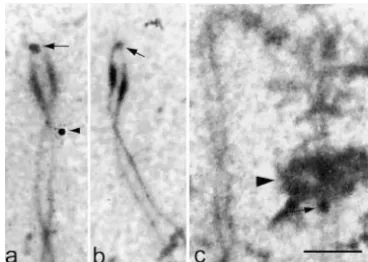
Figure7.—Portions of three maize SCs stained with uranyl The frequency of RNs and SC length: We found a acetate-lead citrate. (a, b) RNs can occur at the very distal tip
positive correlation between total SC set length and the
of an SC (arrows). Stain precipitate (small arrowhead) is much
total number of RNs per SC set in maize withⵑ16% of
darker than RNs and has sharp edges. Thickenings of lateral
elements are present in a and b. (c) Rarely, an RN (arrow) the variation in RN number explained by variations in
can be observed close to the kinetochore (large arrowhead). SC set length (r2⫽0.16; Figure 5). Similar relationships Bar, 1m.
have been reported for humans and certain strains of mice (r2⫽0.13–0.33;Lynnet al.2002), and reanalysis
of the data fromShermanandStack(1995) indicates edu/maps.html). Since no other maize line has been
that a similar relationship also holds in tomato (r2 ⫽
analyzed for RNs, comparisons of RN numbers in
differ-0.13). However, there is only a weak relationship be-ent lines currbe-ently are not possible. However, as an
tween SC set length and number of MLH1 foci for alternative, we compared chiasma frequencies between
males of the mouse inbred strain C57BL/6 (r2⫽0.04),
KYS and three other commonly used inbred lines (W22,
although females of this strain do show a positive rela-B73, Mo17) and a B73/Mo17 hybrid (the cross used to
tionship (Froenickeet al.2002;Lynnet al.2002).Lynn
prepare the IBM map, an intermated B73/Mo17
recom-et al. (2002) showed that the pachytene substage did binant inbred high-resolution molecular map). We
not affect SC set length for humans, and similarr2values
found a 12% difference in average number of chiasmata
(13–16%) for other species suggest that this might be per cell between lines with the least (Mo17) and the
true for these species as well. However, it has been most chiasmata (W22) with the other lines (KYS, B73,
frequently (but not always) noted that SC sets are longer and the B73/Mo17 hybrid) falling in between (Table
in early pachytene than in late pachytene (e.g.,Moses
4). Our results are consistent with those of a number
et al. 1977; Maguire 1978; Gillies 1981). Since it is of investigators who have found differences in
recombi-likely that the number of RNs does not change during nation frequency among inbred lines and crosses for
pachytene (Sherman andStack 1995), any variation maize (e.g.,Pagliariniet al.1986;Beavis andGrant
1991;Fatmiet al.1993;Williamset al.1995;Timmer- in SC length due to pachytene substage could obscure
TABLE 4
Comparison of the mean number of chiasmata for four different inbred lines and a hybrid between two inbred lines (B73/Mo17)
No. of bivalents witha
Inbred No. of cells Mean no. of
line (bivalents) chiasmata (SD) 0 chiasmata 1 chiasmata 2 chiasmata ⱖ3 chiasmata
W22 267 21.2 (1.9) 2 303 1758 607
(2670) (0.1) (11.3) (65.8) (22.7)
B73/Mo17 267 21.0 (1.8) 1 267 1892 510
(2670) (0.0) (10.0) (70.9) (19.1)
B73 270 20.9 (2.2) 10 355 1753 582
(2700) (0.4) (13.1) (64.9) (21.6)
KYS 278 18.9 (2.5) 31 667 1673 409
(2780) (1.1) (24.0) (60.2) (14.7)
Mo17 283 18.5 (1.8) 15 607 1983 225
(2830) (0.5) (21.4) (70.1) (8.0)
Five plants from each line were sampled. The mean number of chiasmata varies significantly between lines (ANOVA,P⬍0.001) as do the variances (Levene’sP⬍0.001).
TABLE 5
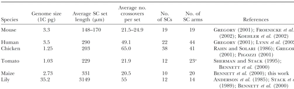
Comparison of SC length from spreads, number of crossovers (based on RNs or MLH1 foci), and number of bivalent arms for male meiotic cells from mouse, humans, tomato, and maize
Average no.
Genome size Average SC set crossovers No. No. of
Species (1C pg) length (m) per set of SCs SC arms References
Mouse 3.3 148–170 21.5–24.9 19 19 Gregory(2001);Froenickeet al.
(2002);Koehleret al.(2002)
Human 3.5 290 49.1 22 44 Gregory(2001);Lynnet al.(2002)
Chicken 1.25 203 65.0 38 41 RahnandSolari(1986);Gregory
(2001);Pigozzi(2001)
Tomato 1.03 229 21.9 12 23a ShermanandStack(1995);
Bennettet al.(2000)
Maize 2.73 331 20.5 10 20 Bennettet al.(2000); this work
Lily 35.2 3149 55 12 14 Andersonet al.(1985);Stacket al. (1989);Bennettet al.(2000)
aThe short arm of chromosome 2 is totally heterochromatic so this arm is excluded here.
the relationship between SC set length and the number tionally large genomes and chromosomes have long SCs and more crossing over (although the relation is not of RNs. With this caveat, these data suggest that variation
in total SC set length within a species is related to varia- proportional), possibly because crossover interference attenuates enough on long SCs to permit additional tion in the total amount of crossing over. Also
support-ing this conclusion is the observation that some female crossover events (see lily, Table 5). Finally, the strength of crossover interference may differ from one group to animals have more crossing over than male animals (e.g.,
zebrafish: Singer et al.2002) as well as longer total SC another;e.g., budding yeast with 16 short SCs hasⵑ100 crossovers (PaˆquesandHaber1999). Thus, while it is set lengths (humans:Bojko1985;WallaceandHulte´n
1985;SpeedandChandley1988;Teaseet al.2002). clear that crossing over is tightly regulated, it is equally clear that a number of factors may be involved in this Does the relationship between SC length and RN
frequency hold between species; i.e., do species with regulation and that not all factors may operate in the same way in different species (AndersonandStack2002). longer total SC lengths necessarily have more RNs? The
answer appears to be no (Table 5). Even though SC How is the rate of crossing over controlled for individ-ual bivalents in a set? It has been recognized for some length is closely correlated with genome size (flowering
plants:Andersonet al.1985; bony fish, reptiles, mam- time that relative chromosome length is positively corre-lated with the level of crossing over and chiasma forma-mals, but not birds:Petersonet al.1994) and genome
size varies greatly among eukaryotes, the number of tion within a species (e.g.,Muller1916;Darlington
1934; Mather 1937). More recently, in-depth studies coding genes is relatively constant. Since most crossing
over takes place within genes, the frequency of crossing have been done on recombination frequency in tomato, chicken, mouse, and maize in which individual bivalents over between species is better correlated with the
num-ber of genes than with total genome size (Thuriaux1977 were identified and examined for RNs or MLH1 foci. All four studies revealed a strong positive correlation and many subsequent reports; Table 5) or with total SC
length. Then why are there differences in the rates of between average SC length and average RN frequency for each bivalent (r2ⱖ0.96 for each species excluding
crossing over between eukaryotic species? First, species
with larger numbers of chromosomes will have more the three shortest SCs from mouse;ShermanandStack
1995;Pigozzi2001;Froenickeet al.2002; this study). crossing over than species with lower numbers of
chro-mosomes due to the obligate crossover between each ho- The rarity of SCs without RNs in maize and tomato (Sherman and Stack 1995) and the rarity of pachy-mologous pair (e.g., chicken, Table 5). Second, the
num-ber of chromosome arms is also positively correlated tene bivalents without Mlh1 foci in mice and chicken (Pigozzi2001;Froenickeet al.2002) illustrate the tight with crossover frequency with an average of one
cross-over per arm for mammals (Pardo-Manuel de Villena control of crossing over that ensures each bivalent (but not necessarily each arm) has at least one crossover andSapienza2001). Tomato and maize fit this general
trend as well (Sherman and Stack 1995; this work). while at the same time apportioning the probability of additional crossovers according to SC length. Thus, there However, both tomato and maize have (short)
chromo-some arms that average less than one RN as well as appear to be at least two levels of control for crossover frequency, one at the level of the cell and another at the (long) arms that average more than one RN (Figure 5;
The distribution and frequency of crossing over along are protected from recombination, possibly including the genes that differentiate maize from teosinte (
Gali-maize SCs: Generally, all 10 maize SCs show similar
patterns of RN distribution (Figure 6). The distal por- nat1988;Doebley1994).
RNs in maize can occur at the very ends of SC arms tions of the arms invariably have the highest average
concentration of RNs, while the frequency of RNs trails (Figures 6 and 7), in contrast to tomato in which no RNs (n ⫽ 9058 observations) were at the ends of SCs off proximally toward the kinetochore, where RNs are
absent. This RN pattern is expected from reports of a (ShermanandStack1995). Inhibition of crossing over at the ends of tomato chromosomes is probably related high distal concentration of chiasmata in maize (Figure
4;Rhoades1950, 1955). This RN pattern also is similar to the presence of prominent dark-staining telomeres with associated repeated DNA sequences that may have to high levels of distal crossing over that have been
reported for two other grass species, wheat (Gill et al. some properties of heterochromatin (ShermanandStack
1995;Zhonget al.1998). In maize, telomere structures 1993, 1996a,b) and barley (Ku¨ nzelet al.2000). In
addi-tion to the general concentraaddi-tion of RNs distally in are not obvious, suggesting that maize telomeres are small and do not interfere with nearby crossing over. maize, there are distinct peaks of RNs involving one or
a few adjacent 0.2-m SC segments. Distinct chromo- The effect of knobs and NORs on crossing over: Heterochromatic knobs are a characteristic feature of somal regions of higher recombinational activity have
been reported also for barley (Ku¨ nzelet al.2000) and maize pachytene chromosomes with the exact number and placement of knobs varying between different lines wheat (Gillet al.1996a). These “hot” regions for
cross-ing over at the chromosomal level (Froenicke et al. (McClintocket al.1981). Knobs are composed of large tandem arrays of 180- and 350-bp repeats (Peacocket 2002) may correspond to hotspots of recombination at
the DNA level, such as the well-known hotspots ata1 al.1981;Ananievet al.1998;Chenet al.2000). Because knobs are heterochromatic, they usually are considered andbz1loci that occur in distal regions of maize
chromo-somes 3 and 9, respectively (Brownand Sundaresan to be recombinationally inert, although variation in the sizes of knobs within populations could be explained 1997;Fuet al.2001, 2002;Yaoet al.2002). However, such
peaks (as well as valleys) in the histograms also may by unequal crossing over within the knobs (Buckleret al.1999). While we were unable to observe knobs due be caused (or exacerbated) by compiling data on the
location of RNs from many different SCs onto an “aver- to dispersion of chromatin in SC spreads, we estimated the position of homozygous knobs on KYS maize SCs age” SC or by sampling errors. The smoothing lines
reduce such variation and show the general trends of using data from Dawe et al. (1992) and Chen et al. (2000). We found that the amount of crossing over at crossing over along the SCs. Determining whether the
individual peaks/valleys are artifactual or represent defi- the location of knobs was either about the same as the average for the SC as a whole (interstitial knobs 5L, 6L, nite positions of elevated or reduced recombination
frequency will require additional study. One method to 7L) or higher than the average (distal knobs 1S and 9S; Figure 6). The knobs on 1S, 9S, and 6L are compara-address this question will be to use fluorescencein situ
hybridization to determine the precise locations of tively small, so they might not be expected to have much effect on RN frequency. However, the knobs on 5L and mapped loci that are known to be hot or cold spots for
crossing over (HarperandCande2000;Sadderet al. 7L are large, and yet they still have appreciable numbers of RNs. This result indicates that knobs have little or 2000;SadderandWeber2002).
Aside from the immediate vicinity of the kinetochore, no effect on reducing the amount of crossing over at their locations on SCs. However, since knobs are hetero-no large segment on any of the maize SCs is completely
free of RNs, but there are segments proximal to kineto- chromatic, the structural relationship of knobs to SC may differ from the structural relationship of euchroma-chores on every SC in which there are only a few RNs
(Figures 6 and 7). A low level of recombination in and tin to SC. The generally accepted model for SC structure has loops of DNA (chromatin) extending from each near centromeres also has been detected by molecular
mapping in Arabidopsis (Copenhaveret al.1998) and lateral element that may include a cohesin core ( Zick-ler and Kleckner 1999; van Heemst and Heyting
in the Festuca/Lolium bivalent (King et al. 2002b). A
reduced level of crossing over proximally is probably 2000;Pelttarriet al.2001;StackandAnderson2001;
Eijpe 2002). We suggest that the DNA in knobs is in related to the centromere effect (Resnick1987) and
to the presence of pericentric heterochromatin in the the form of one to a few long loops of condensed chro-matin that are anchored to a short region of the lateral arms of all maize SCs (Carlson1988;JewellandIslam
-Faridi 1994). Pericentric heterochromatin in maize elements (Figure 8). Knobs, and heterochromatin in general, may have only a few anchoring sequences in does not stain by C-banding, so it may be a “lower grade”
of heterochromatin that permits more crossing over comparison to euchromatic regions. This model agrees with the explanation offered by Stack (1984) for the nearer the centromere rather than the dense blocks of
pericentric heterochromatin in tomato (Shermanand observed underrepresentation of heterochromatin in the length of pachytene chromosomes. In addition, it is
Stack1995). Even so, the pericentric regions of maize
RNs per meiosis for a complete set of KYS maize SCs (Table 2) is equivalent to a total map length of 1025 cM. How do the lengths of the RN maps compare with the classical gene maps and the molecular linkage maps for maize? From Table 2, it is apparent that the genetic and the molecular linkage maps are both roughly twice as long as the RN map. However, when pairwise compar-isons are made between map lengths of individual chro-mosomes (linkage groups) using different maps, all maps are significantly correlated (P⬍ 0.01). The
pre-Figure8.—An SC with euchromatic chromatin loops and
a homozygous heterochromatic knob. Numerous (shaded) dictive value of the correlation is best for the RN map loops of euchromatin extend from the cohesin/lateral ele- compared to the molecular map (r2⫽76%), with lower ment core from regularly spaced attachment sites. The loops
values for the RN map and the gene map (r2⫽ 63%) are shown doubled to represent the two sister chromatids, but
and the gene and molecular maps (r2 ⫽59%). These sister loops may actually extend in opposite directions (Stack
correlations are in the same order but better than the
andAnderson2001). In contrast, knob heterochromatin may
consist of only a few (solid) loops and their attachment sites. same correlations reported for tomato (r2⫽69, 45, and Since crossing over occurs within the context of the SC, the 21%, respectively;ShermanandStack1995). Thus, dif-reduced association of the knob chromatin with the SC would
ferences in crossover frequency between the maps for
greatly decrease, but not eliminate, the amount of crossing
maize seem to apply to all 10 bivalents more or less
over that could occur within the knob itself. However, as shown
equally.
here, RNs that appear to be within the region of the knob
could actually be mediating crossovers between euchromatic The shorter length of the RN map compared to the loops. This would explain why RN frequencies at heterochro- linkage maps could be explained if some RNs are lost matic knobs appear to be about average (or above) for the
(perhaps due to the spreading technique or to RN
turn-SC region where the knobs occur.
over), and, indeed, a small number of maize SCs are without RNs (Table 3). However, this is an unlikely explanation for three reasons:
longer in pericentric heterochromatin than in distal eu-chromatin along tomato SCs (Peterson et al. 1996).
1. The number of univalent pairs from diakinesis chro-Since crossing over in plants and animals occurs in the
mosome squashes matches the number of maize SCs context of the SC, minimal association of knob
chroma-without RNs (⫽0.1%), so this level of failure to cross tin with the SC could sharply reduce crossing over within
over appears to be a normal feature of crossing over homozygous knobs. This model would explain why
ho-in maize whether measured at pachytene or diakho-ine- diakine-mozygous knobs neither alter the local rate of
recombi-sis (Table 3). nation nor add significantly to the length of pachytene
2. The difference in size between RN maps and linkage chromosomes (Rhoades1955;McClintocket al.1981;
maps requires that about half the RNs would have
Stack1984;Jonesandde Azkue1993).
to be lost so that each SC would average two RNs The frequency of RNs in the NOR region in the short
(as actually observed) instead of the “real” four RNs arm of chromosome 6 is slightly lower than that for the
predicted from linkage maps. If RNs were lost at SC as a whole (1.6 RNsvs.2.2 RNs per 0.2-m segment;
random and each RN had a 50% chance of being Figure 6). Crossing over within the NOR also has been
lost, then one would expect ⵑ6% (⫽ 1/24) of the
detected in the Festuca/Lolium bivalent although at a
SCs to have no RNs. This is 60 times more SCs with reduced level compared to other parts of the
chromo-no RNs than were actually observed. some (King et al. 2002b). Considering that NORs are
3. Finally, the RN map is slightly larger than the chiasma made up of tens to thousands of tandem repeats (Heslop
-map (Table 3), so if we are losing half the RNs, we
Harrison2000), NOR DNA may have few anchor
se-must likewise be counting less than half the chias-quences for SCs and a relation to SC similar to that
mata, which again seems unlikely. proposed for knobs and heterochromatin in general.
As a result, crossing over within the NOR itself would So which of the maps most accurately describes the be lower while having little effect on the rate of recombi- amount of crossing over in maize? We argue that the
nation in nearby regions. RN map is the most accurate (at least for male KYS) for
RN maps compared to linkage maps:Two linked genes several reasons:
that recombine 1% of the time during a single meiosis
1. The close agreement between numbers of RNs and are separated by 1 map unit (centimorgan), and 50 map
chiasmata is independent support for the accuracy units correspond to the map distance between two loci
of the RN map (Table 3). in which there is an average of one crossover event per
2. The RN map was prepared using a single inbred line, meiosis. Since each RN corresponds to a crossover event,
whereas linkage maps were prepared using a variety an SC segment that averages one RN per meiosis would
Beadle, G. W., 1933 Further studies of asynaptic maize. Cytologia
3. The RN map is based only on male meiosis, whereas
4:269–287.
linkage maps utilize the products of both male and Beavis, W. D., andD. Grant, 1991 A linkage map based on
informa-tion from four F2 populainforma-tions of maize (Zea maysL.). Theor.
female meioses that may differ in rate and
distribu-Appl. Genet.82:636–644.
tions of crossing over (Rhoades 1941, 1978;
Carl-Bennett, M. D., A. V. CoxandI. J. Leitch, 2000 Angiosperm DNA
son1988). C-values database. http://www.rbgkew.org.uk/cval/database1.
html.
4. The conditions under which the work was performed
Bojko, M., 1985 Human meiosis. IX. Crossing over and chiasma
favors the consistency of the RN map because the
formation in oocytes. Carlsberg Res. Commun.50:43–72.
RN map was produced from plants grown under the Brown, J., andV. Sundaresan, 1997 A recombination hot spot in
the maizeA1intragenic region. Theor. Appl. Genet.81:185–188.
same conditions by the same people using the same
Buckler, E. S. I., T. L. Phelps-Durr, C. S. K. Buckler, R. K. Dawe, instruments and techniques.
J. F. Doebleyet al., 1999 Meiotic drive of chromosomal knobs
5. Several factors have been identified that could lead reshaped the maize genome. Genetics153:415–426.
Carlson, W. R., 1988 The cytogenetics of corn, pp. 259–331 inCorn
to inflated linkage map values (LincolnandLander
and Corn Improvement, edited by G. F.Spragueand J. W.Dudley.
1992;Kinget al.2002a;Knox andEllis2002). Crop Science Society, Madison, WI.
6. Since crossing over takes place in the context of Carpenter, A. T. C., 1975 Electron microscopy of meiosis in Drosoph-ila melanogaster females: II. The recombination nodule—A
re-pachytene chromosomes, it is noteworthy that RN
combination-associated structure at pachytene? Proc. Natl. Acad.
map lengths are better correlated with individual SC Sci. USA72:3186–3189.
lengths than with either genetic or molecular linkage Carpenter, A. T. C., 1979 Synaptonemal complex and recombina-tion nodules in wild-typeDrosophila melanogasterfemales. Genetics
maps. The lower correlations with the linkage maps
92:511–541.
may reflect uneven coverage of markers among the Chen, C. C., C. M. Chen, F. C. Hsu, C. J. Wang, J. T. Yanget al.,
chromosomes. 2000 The pachytene chromosomes of maize as revealed by
fluo-rescence in situ hybridization with repetitive DNA sequences. Theor. Appl. Genet.101:30–36.
Uses of RN maps:RN maps show the physical
distribu-Cleveland, W. S., 1979 Robust locally weighted regression and
tion of crossing over along each bivalent. Such maps
smoothing scatterplots. J. Am. Stat. Assoc.74:829–836.
can be used in a variety of ways. For example, they can Comings, D. E., 1972 The structure and function of chromatin, pp.
237–431 inAdvances in Human Genetics, edited by H.Harrisand
be used to compare gene evolution in regions of the
K.Hirschhorn. Plenum Press, New York.
chromosome with high and low RN frequency (Stephan Copenhaver, G. P., W. E. BrowneandD. Preuss, 1998 Assaying
andLangley1998;Tenaillonet al.2002), to examine genome-wide recombination and centromere functions with Ara-bidopsistetrads. Proc. Natl. Acad. Sci. USA95:247–252.
interference (ShermanandStack 1995;Andersonet
Darlington, C. D., 1934 The origin and behaviour of chiasmata. al. 1999; Froenicke et al. 2002; our unpublished re- VII.Zea mays. Z. indkt. Abstamm.-Vererb. Lehre67:96–114. sults), and to aid in integrating linkage maps with chro- Davis, G. L., M. D. McMullen, C. Baysdorfer, T. Musket, D. Grant
et al., 1999 A maize map standard with sequenced core markers,
mosome structure (Petersonet al.1999;Froenickeet
grass genome reference points and 932 expressed sequence al.2002; our unpublished results). tagged sites (ESTs) in a 1736-locus map. Genetics152:1137–1172. Dawe, R. K., D. A. Agard, J. W. SedatandW. Z. Cande, 1992 Pachy-We thank Ben Burr and Ed Coe for providing KYS seeds. This work
tene DAPI map. Maize Newsl.66:42. was supported by a grant from the National Science Foundation (NSF;
Dawe, R. K., J. W. Sedat, D. A. AgardandW. Z. Cande, 1994 Meiotic MCB-9728673). K.D.H., A.L., and B.B. were supported by grants from
chromosome pairing in maize is associated with a novel chromatin the NSF for Research Experience for Undergraduates. organization. Cell76:901–912.
de la Torre, J., C. Lopez-Fernandez, R. NicholsandJ. Gosalvez, 1986 Heterochromatin readjusting chiasma distribution in two species of the genus Arcyptera: the effect among individuals and populations. Heredity56:177–184.
LITERATURE CITED
Dempsey, E., 1994 Traditional analysis of maize pachytene
chromo-Ananiev, E. V., R. L. Phillips andH. W. Rines, 1998 A knob- somes, pp. 432–441 inThe Maize Handbook, edited by M.Freeling associated tandem repeat in maize capable of forming fold-back and V.Walbot. Springer-Verlag, New York.
DNA segments: Are chromosome knobs megatransposons? Proc. Doebley, J., 1994 Genetics and the morphological evolution of Natl. Acad. Sci. USA95:10785–10790. maize, pp. 66–77 inThe Maize Handbook, edited by M.Freeling
Anderson, L. K., andS. M. Stack, 2002 Meiotic recombination in and V.Walbot. Springer-Verlag, New York.
plants. Curr. Genomics3:507–525. Doyle, G. G., 1994 Inversions and list of inversions available, pp.
Anderson, L. K., S. M. Stack, M. H. FoxandC. Zhang, 1985 The 346–349 inThe Maize Handbook, edited by M.Freelingand V. relationship between genome size and synaptonemal complex Walbot. Springer-Verlag, New York.
length in higher plants. Exp. Cell Res.156:367–378. Eijpe, M., 2002 Homologous recombination, sister chromatid
cohe-Anderson, L. K., A. Reeves, L. M. WebbandT. Ashley, 1999 Distri- sion, and chromosome condensation in mammalian meiosis. bution of crossing over on mouse synaptonemal complexes using Ph.D. Thesis, Wageningen Universiteit, Wageningen, The Neth-immunofluorescent localization of MLH1 protein. Genetics151: erlands.
1569–1579. Fatmi, A., C. G. PoneleitandT. W. Pfeiffer, 1993 Variability in
Ayonoadu, U., andH. Rees, 1968 The influence of B-chromosomes recombination frequencies in the Iowa stiff stalk synthetic (Zea
on chiasma frequencies in black Mexican sweet corn. Genetica maysL.). Theor. Appl. Genet.86:859–866.
39:75–81. Freeling, M., andV. Walbot(Editors), 1994 The Maize Handbook.
Baker, S. M., A. W. Plug, T. A. Prolla, C. E. Bronner, A. C. Harris Springer-Verlag, New York.
et al., 1996 Involvement of mouseMlh1in DNA mismatch repair Froenicke, L., L. K. Anderson, J. WeinbergandT. Ashley, 2002 and meiotic crossing over. Nat. Genet.13:336–342. Male mouse recombination maps for each autosome identified
Bass, H. W., O. Riera-Lizarazu, E. V. Ananiev, S. J. Bordoli, H. W. by chromosome painting. Am. J. Hum. Genet.71:1353–1368.