*Laboratoire Ge´nome, Populations et Interactions, Universite´ Montpellier II, 34095 Montpellier Cedex 05, France,†Laboratoire Ge´ne´tique et
Environment, Institut des Sciences de l’E´volution de Montpellier, Universite´ Montpellier II, 34095 Montpellier Cedex 05, France,
‡Station Biologique de la Tour du Valat, 13200 Arles, France and§I.A.C.R. Long Ashton Research Station, Department of
Agricultural Science, University of Bristol, Bristol BS41 9AF, United Kingdom Manuscript received October 23, 2000
Accepted for publication May 14, 2001
ABSTRACT
Population structure and history have similar effects on the genetic diversity at all neutral loci. However, some marker loci may also have been strongly influenced by natural selection. Selection shapes genetic diversity in a locus-specific manner. If we could identify those loci that have responded to selection during the divergence of populations, then we may obtain better estimates of the parameters of population history by excluding these loci. Previous attempts were made to identify outlier loci from the distribution of sample statistics under neutral models of population structure and history. Unfortunately these methods depend on assumptions about population structure and history that usually cannot be verified. In this article, we define new population-specific parameters of population divergence and construct sample statistics that are estimators of these parameters. We then use the joint distribution of these estimators to identify outlier loci that may be subject to selection. We found that outlier loci are easier to recognize when this joint distribution is conditioned on the total number of allelic states represented in the pooled sample at each locus. This is so because the conditional distribution is less sensitive to the values of nuisance parameters.
P
RESUMED neutral polymorphic loci are commonly andKaplan 1988). Selection acting on any locus hasused in making inferences about patterns of differ- an effect on loosely linked loci, which resembles a
reduc-entiation within or among populations of the same or tion of effective population size (Robertson1961;
Bar-closely related species. For this purpose, genetic dis- ton 1995, 1998). Local adaptation tends to increase
tances (see,e.g.,Nei1972) orWright’s (1951)F-statis- population differentiation at loci where selection acts,
tics are estimated from allele-frequency data. Under and very highFSTvalues may be found at closely linked
particular models of population structure, these param- neutral loci (Charlesworthet al.1997). The
substitu-eters are related to demographic or historical parame- tion of advantageous mutations at a locus may also
re-ters, such as the effective population size, the rate of duce neutral variation at linked loci (Maynard Smith
migration between populations, or the time since the and Haigh1974; Kaplan et al. 1989; Barton 1995).
populations diverged from their common ancestral pop- Similarly, “background selection,” caused by the
selec-ulation. tion against deleterious mutations (Charlesworthet
However, misinterpretations can occur if one is not al.1993; Barton 1995) results in a reduced effective
able to clearly distinguish between the patterns gener- population size for neutral genes in the region of the
ated by random genetic drift or by natural selection. chromosome where this selection is acting. Background
The problem is that selective processes can also affect selection may also increase the apparent population
neutral loci. A locus that is neutral will respond to selec- differentiation (Charlesworthet al.1997).
tion whenever it is in linkage disequilibrium (statistical Therefore, it is of prime interest to identify loci that
association among allelic states at different loci) with are responding to selection to exclude them from the
other loci that are subject to selection. Such associations genetic analysis of population structure or history. It
may arise by chance in small populations (Hill and was recognized early on byCavalli-Sforza(1966) that
Robertson1966, 1968;OhtaandKimura1969). For any form of selection will affect some regions of the
example, stabilizing or balancing selection operating at genome more than others, whereas population history,
a locus tends to maintain an elevated level of variation demography, migration, and the mating system will
af-at closely linked neutral loci (Strobeck1983;Hudson fect the whole genome in the same way. Accordingly,
LewontinandKrakauer(1973) proposed two tests of selective neutrality. Both tests are based on the sampling Corresponding author:Renaud Vitalis, Laboratoire Ge´ne´tique et Envi- distribution of a statisticFˆ, the standardized variance of ronnement, C.C. 065, Institut des Sciences de l’E´ volution de
Montpel-gene frequency, which is an estimator of the parameter
lier, Universite´ Montpellier II, Place Euge`ne Bataillon, 34095
Montpel-lier Cedex 05, France. E-mail: [email protected] FST. Their first test is a goodness-of-fit test comparing
the observed distribution ofFˆ estimates (one estimate true population history consists of repeated branching events or when the connectivity of populations is
un-from each locus) to a2distribution with (n⫺1) d.f.,
even. However, we cannot infer patterns of migration
where n is the number of populations sampled. The
or historical branching and test for the homogeneity of second test is based on the comparison of the observed
the markers with the same data. This is what
Felsen-variance ofFˆ(across loci) denoteds2
F,with the
theoreti-stein(1982) described as the “infinitely many parame-cal variance approximated as
ters” problem. A solution to this problem is to restrict attention to simple but realistic scenarios that may apply
2⫽ kF2
n⫺ 1, (1) to anypairof populations (Robertson1975b;Tsakas
andKrimbas1976). This reduces the number of
param-whereFis the mean value ofFˆaveraged across loci, and
eters in the model. Here, we develop a model of
popula-kis a constant that, according to LewontinandKra- tion divergence. We define population-specific
parame-kauer(1973), should not exceed 2 whatever the under- ters as functions of probabilities of identity for pairs
lying distribution of allelic frequency. The ratio s2
F/2 of genes taken within or among populations. These
should be distributed approximately as a 2/d.f., the
parameters are simply related to the ratio of divergence
number of degrees of freedom being determined by time over effective population size. We construct simple
the number of biallelic loci. estimators of these population-specific parameters. We
However, since populations of the same species share, then examine the expected joint distribution of these
to a certain extent, a common history and since popula- estimators under a wide range of neutral scenarios of
tions are connected through the dispersal of individuals, divergence. This suggests a new method to assess the
Fˆvalues will be correlated across loci. For example, the homogeneity of response of genetic markers to the
his-geographic and historical relationships between popula- torical processes, using empirical data. Finally, we apply
tions may have a hierarchical structure if populations our new method to a data set of allozyme loci from
have been derived from a common ancestral population Drosophila simulanspopulations and compare our results
by a sequence of successive splits. This is the pattern to to those obtained by using Beaumont and
Nich-be expected following the fragmentation of a species ols’(1996) method.
range. The effect of such a population history is always to
increase the expected variance ofFˆ(Robertson1975a,b).
THE MODEL
Moreover, even simple models of divergence by drift
(NeiandChakravarti1977), island models (Neiet al. We consider two haploid populations of constant sizes
1977), or stepping-stone models of dispersal (Neiand N
1 and N2, which completely separated generations
Maryuyama1975) inflate the expected variance, mak- ago from a single population of stationary size N 0. By ing LewontinandKrakauer’s (1973) test unreliable complete separation, we mean that the populations did
in most cases (LewontinandKrakauer1975). not exchange any migrants between the time of the split
More recently, Bowcock et al. (1991) studied the and the present. We do not assume that the common
worldwide human genetic differentiation based on DNA ancestral population was at equilibrium when it split.
polymorphism. Simulating a reasonably well supported Instead, we allow the ancestral population to have gone
evolutionary scenario of divergence, they evaluated the through a bottleneck 0 generations before present
theoretical distribution ofFSTconditional on initial gene (with0⬎ ). Before this, the ancestral population was
frequencies. Among 100 nuclear RFLP markers a num- at mutation-drift equilibrium, with constant sizeNe.
Gen-ber of genes exhibited lower or, more often, higher erations do not overlap. New mutations arise at a rate
variation than expected under neutrality. In an impor- and follow the infinite allele model (IAM). This model
tant article,BeaumontandNichols(1996) proposed of population divergence is illustrated in Figure 1.
a method based on the analysis of the expected distribu- LetQw,ibe the probability that two genes sampled at
tion of FST conditional on heterozygosity rather than random within population i are identical by descent
allele frequency. The conditional distribution, con- (IBD) andQabe the probability that a gene sampled at
structed under an island model of population structure, random from population 1 is IBD to a gene sampled at
is remarkably robust to a wide range of alternative mod- random from population 2. IBD probabilities are
de-els (colonization, stepping-stone). Interestingly, depar- fined as the probabilities that two genes have not
tures from equilibrium do not alter the expected distri- mutated since their most recent common ancestor
bution much whenever FST is ⬍0.5. Yet, unequal (Male´cot1975). The probability that a pair of genes
numbers of immigrants per generation over the whole are IBD is equal to the probability that these genes are
population generated some discrepancies with the sym- identical in state (IIS) whenever the mutation process
metric island model for heterozygosities in the range follows the IAM.
[0.1, 0.5] (see Figure 3d in Beaumont andNichols More generally, letQhdenote the IBD probability of
1996). any pair of genes:h⫽(w,i) when two genes are sampled
within populationi, orh⫽awhen one gene is sampled
Figure1.—A gene genealogy under our model forn⫽10 genes sampled in each population. In this example, the parameter values areN1⫽N2⫽
100,N0⫽500,Ne⫽1000, ⫽50,0⫽150, and
⫽10⫺3.
from each population. It is possible to give an expression
Q0⫽
冮
0r ␥t⫺
N0
e⫺(t⫺)N0dt⫹(1⫺C0)
冮
∞0
␥t⫺0
Ne
e⫺(t⫺0)/Nedt,
forQhas a function of the coalescence time (Slatkin
1991). Under a continuous time approximation (4)
where (1⫺C0)⫽ ␥0⫺·e⫺(0⫺)/N0is the probability that
Qh⫽
冮
∞0 ␥
t
ch(t)dt (2)
the two genes neither coalesce nor mutate in the time
interval ⬍ t ⱕ 0. The first term on the right-hand
(Hudson1990), where ch(t) is the probability of
coales-side of Equation 4 averages over the coalescent events
cence attfor a pair of genes of typeh, and ␥ ⫽(1⫺
occurring during the population bottleneck. During
)2. The waiting time for a coalescent event in a
popula-this time interval ( ⬍ t ⱕ 0) the waiting time for a
tion of sizeNihas an exponential distribution with mean
coalescent event is exponentially distributed with mean
Ni. The IBD probability for a pair of genes in population
N0. The last term in Equation 4 averages over coalescent
ireduces to
events occurring in the ancestral population at muta-tion-drift equilibrium. This last term represents the IBD
Qw,i ⫽
冮
0
␥t Ni
e⫺t/Nidt⫹(1 ⫺C
i)Q0, (3)
probability for two randomly sampled genes in a
station-ary population of sizeNe, which is 1/(1⫹ ), with ⫽
whereQ0is the IBD probability for two genes sampled 2N
e. Solving the integrals in the low-mutation limit
at random from the common ancestral population at (where␥t≈e⫺2t), we find that the solution of Equation
time( just before the split) and (1⫺Ci)⫽ ␥·e⫺/Ni 3 is
is the probability that the two genes neither coalesce
nor mutate in theith population in the time interval 0⬍ Q
w,i ≈
1
i⫹ 1[1⫺e
⫺Ti(i⫹1)]⫹e⫺Ti(i⫹1)·Q0, (5)
tⱕ . The first term on the right-hand side of Equation 3
is the probability that the two genes coalesce in the time wherei⫽2
NiandTi⫽ /Ni. The value ofQ0is given
period 0⬍ tⱕ and are IBD. Following Equation 2, by the solution of Equation 4,
the IBD probability for a pair of genes sampled at
ran-dom from the common ancestral population just before Q
0 ≈ 1
0⫹ 1
[1⫺e⫺T0(0⫹1)]⫹e⫺T0(0⫹1)
冢
1 ⫹1
冣
, (6)where0⫽2N0andT0⫽(0⫺ )/N0. The probability During this period, all the coalescent events are sepa-rated by exponentially distributed time intervals, with for a gene in population 1 to be IBD with a gene in
population 2 is just given by meansN1/(n1
2) in population 1 andN2/(n22) in population
2 (see Equation 3). At time, the numbern0of lineages
Qa⫽ ␥Q0. (7) that remain represents the ancestors of all the genes
sampled in populations 1 and 2. The genealogy of these Obviously, two such genes cannot coalesce during the
lineages is generated for the time period [,0], and all
generations between the moment of divergence and
the coalescence events are separated by exponentially the present. They are IBD only if their respective
ances-distributed time intervals, with mean N0/(n0
2) (see the
tors are IBD when populations 1 and 2 diverge and,
first term in the right-hand side of Equation 4). At time furthermore, if they do not undergo mutation during
0, the lineages that remain are the ancestors of all the the divergence. Now, it is useful to consider the
param-genes sampled in populations 1 and 2. The genealogy eter
of thesenegenes is generated for the period [0,⫹∞],
with all coalescent events separated by exponentially
Fi⫽
Qw,i⫺Qa
1⫺Qa
. (8)
distributed time intervals with mean Ne/(n2e) (see the
second term in the right-hand side of Equation 4). Once
It is worth noting that the weighted sum ofFiover the
the complete genealogy is obtained, the mutation events two populations gives the intraclass correlation for the
are superimposed on the coalescent tree of lineages. In probability of identity by descent for genes within
popu-the results that follow, each artificial data set consisted lations relative to genes between populations. This is of
of two (haploid) samples of size n ⫽ 100, one from
particular interest, because the properties of the
in-population 1 and the other from in-population 2. traclass correlations for the probability of identity in
Simulation results: By calculating the estimators Fˆ1
state (“IIS correlations”; CockerhamandWeir 1987)
andFˆ2for each of these artificial data sets, it was possible
can be deduced from the properties of the
correspond-to obtain a close approximation correspond-to the expected distri-ing intraclass IBD correlations in the low-mutation limit
bution of these estimators (seeappendix for details).
(Rousset1996). Indeed, such ratios of identity
proba-Figure 2 shows this expected joint distribution ofFˆ1and
bilities of the form of Equation 8 give the same
low-Fˆ2for various combinations of the nuisance parameters
mutation limit, whether one considers the infinite allele
andT0. In this case, the “true” branch lengths were
model or other mutation models (Rousset1996, 1997).
T1⫽T2⫽0.1 (henceF1 ⫽F2≈0.0953). The expected
If we neglect new mutations arising during the
diver-value of the estimator Fˆ1 (respectively Fˆ2) was always
gence process,Qareduces toQ0andQw,i⫽Ci(1⫺Q0)⫹
close to the value of the parameterF1(respectivelyF2).
Q0. Thus
One can show that, by construction, the points (Fˆ1,Fˆ2)
lie within the upper-right triangle with vertices (1, 1),
Fi≈ 1⫺ e⫺Ti. (9)
(⫺1, 1), and (1,⫺1). The joint distribution of these two
Note that Equation 9 gives a well-known result when statistics has a negative correlation. Most importantly, it
both daughter populations are assumed to have the is clear from this figure that the joint distribution ofFˆ
1
same sizeN, so thatF1 ⫽ F2 ⫽ F≈ 1⫺ e⫺/N(see,e.g., and Fˆ
2 depends strongly on the nuisance parameters,
Reynolds et al. 1983). Hereafter, the parameter Ti is even though their expectations remain close to the true
referred to as the “branch length” of populationi.An values ofF
1 andF2.
important result is that, in the low-mutation limit, the It can be seen that, for smaller values ofT0, the joint
new parameters F1andF2 do not depend on the “nui- distribution becomes tighter asincreases. On the other
sance parameters” or T0. This suggests that a simple hand, for larger values of , the distribution is found
moment-based estimator Tˆi of branch length can be to widen asT
0increases. In both cases, it is the level of
derived as variation that remains before divergence that is crucial
in shaping the joint distribution. With smalland large
Tˆi⫽ln(1 ⫺Fˆi), (10)
T0, the lineages coalesce rapidly before the divergence,
whereFˆiis an estimator ofFi(seeappendixfor details). and the number of distinct mutations (allelic states)
that can be maintained is small. In this case, the variance of the estimates of populations branch lengths is large,
PROPERTIES
as illustrated by the wide joint distribution ofFˆ1andFˆ2.
Therefore, the joint distribution ofFˆ1andFˆ2is not ideal
Simulation procedure:For each set of parameter
val-ues, a sequence of artificial data sets was generated using for investigating the homogeneity of response of a set
of molecular markers to the genealogical processes.
In-standard coalescent simulations, as described by, e.g.,
Hudson (1990). The simulations were performed as deed, other factors such as heterogeneous mutation rates across loci may be invoked to explain disparities follows (see Figure 1 for an illustrated example of one
simulated genealogy). For each population, the geneal- of branch length estimates among markers. Fortunately,
this problem can be overcome by considering the joint
ogy of a sample ofnigenes is generated for a period of
Figure 2.—Expected distribution of pairs ofFˆ1andFˆ2estimates for wide ranges
of values of the nuisance parameters ⫽ 2Ne and T0. Ti ⫽ /Ni is 0.10 for both daughter populations (with ⫽50 andN1⫽
N2 ⫽ 500), giving an expected value Fi ≈ 0.0953, as indicated by the dotted lines. For all parameter sets, ⫽10⫺4andN
0⫽1000.
One hundred individuals are sampled in each daughter population. The light gray area defines a region in which 95% of the simulated points are expected to lie (see
appendixfor details).
numberkof allelic states in the pooled sample at each 3. The expected joint distribution ofFˆiandFˆjis
gener-ated by performing 10,000 coalescent simulations locus. Figure 3 shows the estimated joint distribution
forT1⫽T2⫽0.1 (henceF1⫽F2≈0.0953), conditioned for a given set of nuisance parameter values. This is
repeated using a wide range of values for the
nui-on k ⫽ 4. The combinations of nuisance parameter
values are the same as in Figure 2. sance parameters. In the D. simulans data set
dis-cussed below, all the pairwise combinations forand
The expected joint conditional distribution appears
to be almost independent on the nuisance parameters. T0 were performed, with ⫽1, 5, or 10 and T0 ⫽
0.01, 0.1, or 1. Thus, a total of 90,000 coalescent
So, given the observed values for the parametersF1and
F2, and given the number of alleles in the sample, one simulations were performed in this example. The
simulated sample sizes are chosen to be representa-can obtain the conditional joint distribution, and then
a high probability region, that should contain 95% of tive of those actually realized in the real data set.
4. For each expected joint distribution ofFˆiandFˆj, we
the observed measures of pairwiseFˆi’s values. This result
provides the justification for using the conditional distri- construct all the distributions, conditional on the
number of allelic stateskin the pooled sample, for
butions to analyze the homogeneity in the patterns of
genetic differentiation revealed by a (large) set of k ⫽ 2, 3, . . . (the pooled sample is the sample
obtained by pooling the samples from populationsi
markers.
andj). Remember, there is one expected
distribu-tion for each set of nuisance parameter values. For
APPLICATIONS each conditional distribution, we identify the “high
probability” or “high density” region, in the range In this section, we present a methodology for
identi-of the pointsFˆi and Fˆj, where 95% of the data are
fying outlier loci by a pairwise analysis of populations.
expected to lie (see appendixfor the construction
For each pair of populations (i,j), we suggest the
follow-of this high probability region). ing protocol:
5. For each value of the number of allelic states in the
1. For all loci, the statisticsFˆiandFˆjare computed (see pooled sample, we superimpose a scatter plot of the
appendix). observed data points (pairs ofFˆ
1andFˆ2values) over
2. The parametersFiandFjare estimated as the averages an outline of the 95% high probability region to
among loci weighted by the heterozygosities (1 ⫺ identify outlier loci.
Qˆi) and (1⫺ Qˆj), respectively (seeappendix). This
D. simulansdata set:We applied this method to aD.
corresponds to the weighting of loci suggested by
simulansdata set, described inSinghet al.(1987) and
WeirandCockerham(1984) for the multilocus
Figure 3.—Expected distribution of pairs ofFˆ1andFˆ2estimates conditioned on
a number of alleles in the sample equal to four. As in Figure 1, wide ranges of values were used for the nuisance parameters. The dotted lines indicate the expected values forF1andF2.
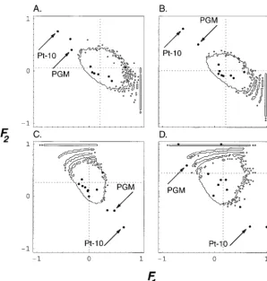
provided by R. S. Singh and R. A. Morton. Among 111 and D). In all pairwise comparisons that included the
French population, these two loci fell either outside, or allozyme loci, 43 were found to be polymorphic in the
five populations studied in Europe and Africa. The sam- on the edges of the 95% high probability region.
In all the pairs that included the population from ples consisted of isofemale lines maintained in the
labo-ratory. The haploid sample sizes ranged from n ⫽ 26 Congo, two loci coding respectively for the larval
pro-tein-10 (Pt-10) and the phosphoglucomutase (PGM)
ton⫽ 55. Figure 4 shows the analysis performed on a
particular pair of populations (France and Tunisia). were found to lie outside or on the limit of the 95%
high probability region (Figure 5). The locus coding
The multilocus estimates of the parametersF1(French
population) andF2(Tunisian population) were 0.0064 for the larval protein-10 systematically gives a longer
estimated branch length for this African population and 0.0617, respectively. The expected distributions
with these averaged values, conditioned on the number than do all other loci, while it gives similar branch
lengths to other loci for the other populations. This of alleles in the pooled sample, are plotted with the
actual monolocus pairwise (Fˆ1,Fˆ2) estimates. suggests that genetic variation was severely reduced by
a factor other than genetic drift in this African popula-In the great majority of cases, the points fall within
the 95% confidence region. With 43 loci we would ex- tion. The locus coding for phosphoglucomutase gives
a longer branch length estimate than the other loci in
pect two (0.05⫻ 43≈ 2) to lie outside the region by
chance. But considering the joint distributions for loci three cases (Figure 5, A–C) and a shorter one in one case
(Figure 5D). The locus coding for phosphoglucomutase with three or more alleles, we found 4 loci that clearly
lie outside. Caution is required in the case of loci that was also found to lie outside the limit of the 95% high
probability region in all the pairs that included the popula-lie on the borders of the possible range (Figure 4B).
These correspond to loci that have an allele fixed in one tion from Seychelle Island (Figure 6). To strengthen our
presumption that these loci were outside the limit al-population. Slight variations in the nuisance parameters
can increase or decrease the relative proportion of loci lowed by a neutral model, we checked whether these
loci also lie outside the limit of the 99% high probability that may fix one allele in a population. Indeed, we
found some conditions under which the 95% envelope region. The same results were obtained. For these loci,
we did not find any plausible neutral scenario of diver-contained these 2 loci. This problem can remain even
when we condition on the observed number of alleles. gence by drift that could provide such a scatter of points.
We thus conclude that natural selection may have acted On the other hand, 2 other loci (coding for glutamate
pyruvate transaminase and carbonic anhydrase-3) are on these loci or on closely linked regions within the
Figure4.—Fˆ1andFˆ2values estimated from 43
loci inDrosophila simulansfor the pairwise compar-ison of the populations from France (n⫽55) and Tunisia (n⫽52). nis the number of isofemale lines typed for each enzymatic system (haploid sample size). Each locus is represented with a solid dot. The averaged values are Fˆ1⫽ 0.0064
andFˆ2⫽0.0617 as indicated by the dotted lines.
Thin solid lines enclose a region in which 95% of the simulated data points are expected to lie. Four distributions are shown, conditioned on the number of allelic states kin the whole sample: (A) expected distribution of pairwiseFiestimates conditioned onk⫽2; (B) withk⫽3; (C) with k⫽4; and (D) withk⫽5. Solid arrows indicate outlier loci. The loci coding for glutamate py-ruvate transaminase (GPT) and carbonic anhy-drase-3 (Ca-3) are shown, respectively, in C and D.
We are more cautious about claiming that the loci An alternative approach would be to develop a new
model of population divergence that allows subsequent coding for glutamate pyruvate transaminase and
car-bonic anhydrase-3 were or are subject to selection. migration after separation. But if we want to make
infer-ences about a more realistic (and hence a more com-These loci are clear outliers in some pairwise
compari-sons involving the French population but fall just within plex) model of divergence, then we need to distinguish
between the pattern of genetic differentiation that re-the limits of re-the confidence region in ore-ther
compari-sons. Moreover, when considering 99% confidence re- sults from (i) recent separation followed by very little
migration or (ii) ancient separation followed by a mod-gions instead of 95% confidence remod-gions, some loci were
no longer detected as outliers but rather as lying on the erate amount of migration. This is a difficult task, which
would require more powerful methods for inferring edges of the confidence limit. The locus coding for
isocitrate dehydrogenase-1 was found to be an outlier parameter values (e.g., maximum likelihood; see
Niel-senandSlatkin2000) that would be much more time in three (out of four) pairs that included the population
from Seychelle Island. Overall, six more loci were de- consuming. Further, note that Nielsen and Slatkin
(2000) assume that the mutation rate is zero. tected as outliers in single pairwise comparisons only.
Therefore, we should be very cautious about consider- So, we are interested in testing if our method (which
assumes evolution in complete isolation after diver-ing those latter loci as bediver-ing under selection. Indeed,
if a locus has responded to selection in one particular gence) is undermined when applied to pairs of
popula-tions that still exchange genes after divergence. It contemporary population since it became isolated, then
we expect this locus to show up as an outlier in all should be borne in mind that gene flow, like genetic
drift, affects the whole genome in the same way. We (or most) comparisons involving this population. This
pattern is exactly what we found for the two loci coding generated artificial data sets under neutral models of
population divergence, including high mutation rates for larval protein-10 and phosphoglucomutase in the
Congo and Seychelle Island populations. and moderate levels of migration between populations.
We used a modified version of the algorithm described Evaluating the robustness of this method to the
as-sumptions of the model:In the data set discussed above, by Hudson(1990), which accounts for symmetric mi-gration between populations. For the period of time
it is likely that the populations ofD. simulanshave
ex-changed migrants after divergence. More generally, one ranging from present togenerations in the past,
con-sidering populations 1 and 2 altogether, the waiting can wonder whether complete isolation and divergence
Figure5.—Fˆ1andFˆ2values estimated from 43
loci inDrosophila simulansfor all the pairwise com-parisons involving the population from the Congo (n⫽45). (A) Expected distribution for the popu-lations from France (n ⫽ 55) and Congo. (B) Tunisia (n⫽52)vs.Congo. (C) Congovs.Cape Town, South Africa (n ⫽ 32). (D) Congo vs. Seychelle Island (n⫽ 26). All distributions are conditioned onk⫽4. Each locus is represented with a solid dot. Dotted lines give the expected values forFˆ1andFˆ2. For each expected conditional
distribution, solid arrows indicate the loci coding for the larval protein-10 (Pt-10) and phosphoglu-comutase (PGM).
drawn from an exponential distribution with mean hallet al.1990) to determine if the distribution of the
number of detected outlier loci was shifted to the right
N1N2/[N2/(
n
21) ·N1/(
n
22)⫹m(n1⫹n2)N1N2], wheremis
the backward migration rate (Nordborg2001). Condi- of 2.5 (one-tailed test).
Table 1 shows the total observed number of outlier tionally on the occurrence of one event, two genes
co-alesce in population 1 (respectively population 2) with loci (mean and median over 20 independent simulated
data sets) detected for a range of nuisance parameter probability N2/(n21)/[N2/(
n
21) · N1/(
n
22) ⫹ m(n1 ⫹ n2)
N1N2] (respectivelyN1/(
n
22)/[N2/(
n
21) ·N1/(
n
22)⫹m(n1⫹ values (low and high mutation rates, short or long
diver-gence by random drift, with or without migration). In
n2)N1N2]) or one gene migrates from population 2 to
population 1 (respectively from population 1 to popula- no case could we reject the null hypothesis that the
expected number of outlier loci detected by our method tion 2) with probabilitym·n1/[N2/(n21) ·N1/(
n
22)⫹m(n1⫹
n2)N1N2] (respectivelym·n2/[N2/(
n
21) ·N1/(
n
22)⫹m(n1⫹ was equal to 2.5 (against the alternative hypothesis that
the expected number of outliers was⬎2.5). Thus, our
n2)N1N2]; seeStrobeck1987;Takahata1988;
Nord-borg2001). Then, for the period [,⫹∞], the coalescent approach is conservative in the sense that the 95%
con-fidence region contains at least 95% of the loci gener-process was generated as previously described (see also
Figure 1). ated by a truly neutral model. At the level of 5% we do
not (falsely) detect any more than 5% of outlier loci in For each set of parameters, we generated 20 data sets
composed of two samples (n1⫽n2⫽50) of 50 loci each. a sample of neutral markers (type I error).
Comparison with Beaumont and Nichols’ (1996)
The parameter values are given in Table 1. For each
data set, we applied our method as described above. method: We also applied Beaumont and Nichols’
(1996) procedure to theD. simulansdata set. Based on
We generated joint distributions, conditional on the
number of alleles, according to the actual numbers of a preliminary examination of the data, three loci
(cod-ing for␣-fucosidase, dipeptidase-1, and mannose
phos-alleles in each sample. For all sets of parameters, we
grouped loci with eight alleles and more in a single phatase isomerase) were found to lie outside the 95%
confidence region of the conditional joint distribution class. The number of joint conditional distributions
gen-erated per artificial data set (i.e., the number of classes of FˆST and mean heterozygosity. The percentiles were
determined as described in Beaumont and Nichols
for different numbers of alleles) ranged from three to
seven. For each data set, over all the joint conditional (1996). Surprisingly, none of these three loci were
de-tected as outliers using our method. There may be sev-distributions taken together, we expected to detect
0.05 ⫻ 50⫽ 2.5 outlier loci, just by chance. We per- eral reasons for this.
We suspect that, in the present case, the inclusion of
Menden-Figure6.—Fˆ1andFˆ2values estimated from 43
loci inDrosophila simulansfor all the pairwise com-parisons involving the population from the Seychelle Island (n⫽26). (A) Expected distribu-tion for the populadistribu-tions from France (n⫽ 55) and Seychelle Island. (B) Tunisia (n⫽ 52) vs. Seychelle Island. (C) Congo (n⫽45)vs.Seychelle Island. (D) Cape Town, South Africa (n⫽32)vs. Seychelle Island. Distributions in A and C are conditioned onk⫽4 and distributions in B and D are conditioned onk⫽3. Each locus is repre-sented with a solid dot. Dotted lines give the ex-pected values for Fˆ1 and Fˆ2. For each expected
conditional distribution, solid arrows indicate the locus coding for phosphoglucomutase (PGM).
a very distant insular population (Seychelle Island) may a local scale, pairwise comparisons of populations are
more likely to be efficient for detecting outlier loci. bias their analysis. Indeed, populations heterogeneous
with respect to their demographic parameters (effective population sizes and migration rates) were shown to
DISCUSSION
strongly affect their method (BeaumontandNichols
1996). Isolation (low migration rates) together with Using population-specific estimators of branch
lengths:Conventional pairwise genetic distances or pair-population bottlenecks can introduce a further bias.
Consider as an extreme case the fixation of a private wise measures of population differentiation are based
on the assumption that the sizes of populations are allele at some locus in one population. This may be
unexpected for a polymorphic locus in a mutation- equal and constant through time or that dispersal, if any,
is symmetric. For example, the pairwiseFSTparameter is
migration-drift equilibrium model, unless there is a
strong asymmetry, with some populations being smaller defined as a ratio of identity probabilities within and
among populations. But the within-population term is and receiving less immigrants than others. However,
this is not unexpected for a model of separation and taken as an average over the pair of populations. Thus,
the definition of the parameter implicitly assumes that isolation, where there were population bottlenecks. This
may boost theFSTestimate at some locus and thus ex- both populations share the same demographic
parame-ters.WeirandCockerham’s (1984) estimatorofFST
clude it from the 95% high probability region. So,
iso-lated populations should probably be excluded from is constructed to have low bias and variance, assuming
that the populations are independent replicates of the
BeaumontandNichols’ (1996) analysis.
Moreover, in general, the loci that were outliers in same stochastic process. This means that populations
are supposed to have the same size and that they do
our analysis gave small values of (global)FST. But from
the shape of the joint distribution ofFSTand heterozygos- not exchange migrants. Without these assumptions,
would be a complex function of unequal
(within-popu-ity, it seems thatBeaumontandNichols’ (1996)
analy-sis is likely to detect outlier loci that exhibit unusually lation) identity probabilities.
In contrast, the Fˆi parameters defined here make
largeFST values. However, a process that would cause
an apparent decrease of genetic variation at one locus sense even when the populations are of unequal size.
The only assumption we make is that when the two in a single local population, without leading to a
de-crease of the variation over all populations, would not populations have separated, they remain completely
iso-lated. From the estimation ofFi’s for a pair of
popula-be detected inBeaumontandNichols’ (1996)
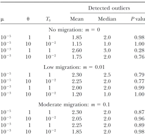
TABLE 1 selection in the population from Congo, one of which was also probably subject to selection in the population Results from applications to various divergence scenarios
from Seychelle Island. We concluded that the distribu-tion of variability at these loci may have been shaped
Detected outliers
by forces other than mutation and drift. Furthermore,
T0 Mean Median Pvalue we identified two other loci that either lie on the edges
or fall just outside the high probability region of the
No migration:m⫽0
expected conditional distribution in the French
popula-10⫺5 1 1 1.85 2.0 0.98
10⫺5 10 10⫺2 1.15 1.0 1.00 tion, although we are more cautious about these latter
10⫺3 1 1 2.60 3.0 0.28
loci. It is noteworthy that our estimation of the density
10⫺3 10 10⫺2 1.75 2.0 0.76
of Fˆi parameters (seeappendix) is discontinuous,
be-cause of the discrete nature of the data (the allele
Low migration:m⫽0.01
counts). This is particularly true when the number of
10⫺5 1 1 2.30 2.5 0.79
alleles on which the distribution is conditioned is small
10⫺5 10 10⫺2 2.25 2.0 0.77
10⫺3 1 1 2.00 2.0 0.99
(for a given set of parameters, the lower the number
10⫺3 10 10⫺2 1.20 1.0 1.00
of allelic states, the more discontinuous the null distri-bution; see Figure 4). Using discrete distributions is
Moderate migration:m⫽0.1
clearly preferable to using some (unnecessary)
continu-10⫺5 1 1 2.30 2.0 0.87
ous approximations to it. Moreover, whenever the null
10⫺5 10 10⫺2 2.05 2.0 0.96
10⫺3 1 1 2.25 2.0 0.89 distribution is based on the same number of allelic states
10⫺3 10 10⫺2 1.85 2.0 0.98
and the same number of genes as in the sample, there is no tendency for loci to show up as outlier just because
For all sets of parameters, 50 loci were scored among 100
of the discrete nature of the distribution (i.e., a locus
haploid sampled individuals (50 in each population). The
mean (and median) number of outlier loci detected is tabu- cannot, by construction, show up between arc-shaped
lated. We provide the P values of Wilcoxon’s signed-rank areas located at the edge of some distributions). Yet, tests, performed on the distributions of detected outliers, to when an apparent outlier lies very close to the 95% determine whether this distribution was shifted to the right
high probability region, it is highly advisable to check
of 2.5 (one-tailed test).
whether this locus also lies outside the 99% high proba-bility region.
The main criticisms of Lewontin and Krakauer’s
these branch length estimates is inversely proportional
to the ratio of effective population sizes. Thus, these (1973) attempts to interpret across-loci heterogeneity
ofFSTvalues arose from their failure to consider allele
estimates may be seen as measures of the intensity of
genetic drift that has occurred since population diver- frequencies as random variables, whose distribution
de-pends on the underlying model of population structure gence. The main drawback to this approach is that when
estimates of IIS probabilities are smaller within popula- and history. Indeed, uneven patterns of dispersal among
populations (NeiandMaryuyama1975) or sequences
tions than among them (i.e., Qˆw,i ⬍ Qˆa), Fˆi becomes
negative, and the moment-based estimator of branch of population splits within the species (Robertson
1975a,b) may strongly undermine the approach.
Lew-length fails. Although this can arise just by chance for
some loci, averaging Qˆ estimates over loci reduces the ontinandKrakauer(1975) acknowledged that their
tests might be limited to situations where the true popu-problem.
Provided that we obtain good estimates of branch lengths lation structure did not depart too much from the island
model. for a pair of populations (which requires the pooling
of information from many independent loci), we may However, conditioning the distribution ofFSTon the
heterozygosity (Beaumont andNichols 1996) or on
be able to evaluate the consistency of locus-specific
esti-mates. Indeed, the joint distribution of branch length gene frequency for biallelic loci (Bowcocket al.1991)
was shown to give surprisingly robust results, in the sense estimates, conditioned on the number of alleles in the
pooled sample, depends only weakly on nuisance pa- that strong departures from the model assumptions do
not alter the distribution very much. The strongest effect rameters of the simple model of divergence by drift. In
particular, this conditional distribution is not sensitive on the joint expected distribution ofFSTand
heterozy-gosity occurs when populations are heterogeneous with to departures from mutation-drift equilibrium before
isolation or to differences in mutation rates. respect to their demographic parameters (Beaumont
andNichols1996), for example, when populations are Detection of selection acting on genetic markers:We
saw from the analysis of the D. simulans data set that founded by very different numbers of individuals or
when populations are arranged in an irregular stepping-the great majority of loci always fall in stepping-the confidence
region of the conditional pairwise distributions of stone lattice. However,BeaumontandNichols(1996)
considered a large numberdof subpopulations in the
branch length estimates, while some loci do not. Overall,
ever, this is not feasible, as the range of models that
Nichols(1996) in determining whether mutation has
an effect onFSTor not. It was shown that, considering incorporate selection is very large.
An important task for the future is to consider a more
smaller numbers of populations,FST estimates may be
reduced by mutation, especially with a stepwise muta- general neutral model of the divergence of two
popula-tions, where gene flow may continue after the moment
tion model (seeFlintet al.1999). Withd⫽100 islands,
the sets of parameters used inBeaumontandNichols of “separation.” It is also desirable to extend this
ap-proach to more elaborate neutral models, incorporating (1996) did not account for any case where mutation
may depressFST. recombination. More sophisticated estimators of the
di-vergence parameters (branch lengths) would then be
As already suggested byTsakasandKrimbas(1976),
restrictingLewontinandKrakauer’s (1973) approach required. We assumed that the mutation process follows
the IAM and we allowed a wide range of possible muta-to pairs of populations removes all kinds of dependence
on the unknown population structure. Indeed, whatever tion rates. In the IAM, genes that are identical in state
are also identical by descent. This may not be the case their history, two populations ultimately descend from
a single ancestral one in the past. Still, nuisance parame- with other mutation models such as with theK allele
or stepwise mutation processes, which can produce IIS
ters may broaden the joint distribution of pairwiseFi’s
(Figure 2). However, conditioning on the number of genes that are not IBD (homoplasy). The IAM is
proba-bly an adequate model for allozyme data. It is certainly alleles (Figure 3) also gives distributions that are robust
enough to variations in the values of nuisance parame- not so appropriate for potentially more variable
mark-ers, such as microsatellites. Recent studies revealed that ters. It is obvious that, for each analysis of a pair of
populations, we deliberately discard the information the processes of mutation of microsatellite markers may
be more complex than previously thought and may vary brought by other populations, which may decrease the
power of the method (TsakasandKrimbas1976). But greatly among loci (EstoupandAngers1998).
Further-we believe that this enables us to explain a wider range more, the effect of homoplasy on measures of
popula-of patterns than any symmetrical model, such as the tion subdivisions is not simple (Rousset1996).
There-island model. In this respect, our approach is conserva- fore, further studies should be conducted to test the
tive. Moreover, we found that low or moderate gene application of our method across different classes of
flow did not undermine our approach, in the sense that nuclear markers that differ in processes of mutation.
the probability of falsely detecting a neutral locus as an Clearly, if a whole class of marker loci, which are known
outlier (type I error) is no more than 5% (Table 1). to have a very distinct mutation process, are identified
We compared the performance of our method to that as outliers by our analysis, then this class of markers
ofBeaumontandNichols(1996), using the empirical should be interpreted with caution.
data from Singh et al. (1987) and Choudhary et al. If we could identify those marker loci that responded
(1992). We further tested whether our method would to selection during the process of divergence, then we
falsely reject neutral loci (type I error) any more than may be able to obtain improved estimates of the
parame-expected, under a wide range of nuisance parameter ters of population structure and history by excluding
values (see Table 1). In particular, since the method these loci (Rosset al.1999). Our method differs from
assumes that the mutations arising after divergence can previous ones in allowing selection to be detected in
be neglected, we checked that high mutation rates do particular populations and in some pairwise
compari-not weaken the approach. sons but not others. This opens up the possibility that
We found that patterns such as those identified in, markers may be discarded only in the analysis of those
e.g., the Tunisiavs.Congo data set as evidence of selec- populations where there is evidence that they have
re-tion can be produced by “neutral models,” where the sponded to selection. It is also of interest to use this
coalescent process occurs independently at each locus. approach to screen the genome for regions that have
Indeed, similar scatters of points could be obtained responded to strong selection in the recent past. If
popu-whenever the parametersFˆ1andFˆ2vary across loci, hav- lations have diverged phenotypically and if this has been
ing particularly high values at certain loci (results not caused by selection, then it may even be possible to
shown). Models of this type provide a rough approxima- identify candidate regions for the quantitative trait loci
tion to models of unlinked neutral loci, some of which underlying this adaptive divergence.
were strongly influenced by selection (remembering
We are very grateful to R. S. Singh and R. A. Morton for providing
that the effect of selection resembles a reduction in the theDrosophila simulansdata set. We thank I. Olivieri for helpful
com-effective population size experienced by these loci, as ments on a previous draft of this manuscript and S. Billiard for valuable
discussions about the structured coalescent. We are grateful to two
Nei, M.,andT. Maryuyama,1975 Lewontin-Krakauer test for neu-anonymous reviewers for their constructive comments. This work was
tral genes. Genetics80:395. funded by contract no. BIO4-CT96-1189 of the Commission of the
Nei, M., A. ChakravartiandY. Tateno,1977 Mean and variance European Communities (DG XII) to P.B., and R.V. was also partially
ofFSTin a finite number of incompletely isolated populations.
funded by the Fondation Sansouire. This is publication no. 2001-045
Theor. Popul. Biol.11:291–306.
of the Institut des Sciences de l’E´ volution de Montpellier. Nielsen, R.,andM. Slatkin,2000 Likelihood analysis of ongoing gene flow and historical association. Evolution54:44–50.
Nordborg, M.,2001 Coalescent theory, pp. 179–212 inHandbook of Statistical Genetics, edited byD. J. Balding, M. BishopandC. LITERATURE CITED
Cannings.John Wiley & Sons, Chichester, UK.
Ohta, T., and M. Kimura,1969 Linkage disequilibrium due to
Barton, N. H.,1995 Linkage and the limits to natural selection.
Genetics140:821–841. random genetic drift. Genet. Res.13:47–55.
Reynolds, J., B. S. WeirandC. C. Cockerham,1983 Estimation of
Barton, N. H.,1998 The effect of hitch-hiking on neutral
genealo-gies. Genet. Res.72:123–133. the coancestry coefficient: basis for a short term genetic distance. Genetics105:767–779.
Beaumont, M. A.,andR. A. Nichols,1996 Evaluating loci for use
in the genetic analysis of population structure. Proc. R. Soc. Lond. Robertson, A.,1961 Inbreeding in artificial selection programmes. Genet. Res.2:189–194.
Ser. B263:1619–1626.
Bowcock, A. M., J. R. Kidd, J. L. Mountain, J. M. Hebert, L. Caro- Robertson, A.,1975a Gene frequency distribution as a test of selec-tive neutrality. Genetics81:775–785.
tenutoet al., 1991 Drift, admixture, and selection in human
evolution: a study with DNA polymorphisms. Genetics88:839– Robertson, A.,1975b Remarks on the Lewontin-Krakauer test. Ge-netics80:396.
843.
Cavalli-Sforza, L. L.,1966 Population structure and human evolu- Ross, K. G., D. D. Shoemaker, M. J. B. Krieger, J. DeHeerandL. Keller,1999 Assessing genetic structure with multiple classes tion. Proc. R. Soc. Lond. Ser. B164:362–379.
Charlesworth, B., M. T. MorganandD. Charlesworth,1993 of molecular markers: a case study involving the introduced fire antSolenopsis invicta.Mol. Biol. Evol.16:525–543.
The effect of deleterious mutations on neutral molecular
varia-tion. Genetics134:1289–1303. Rousset, F., 1996 Equilibrium values of measures of population subdivision for stepwise mutation processes. Genetics142:1357–
Charlesworth, B., M. Nordborg andD. Charlesworth, 1997
The effects of local selection, balanced polymorphism and back- 1362.
Rousset, F.,1997 Genetic differentiation and estimation of gene ground selection on equilibrium patterns of genetic diversity in
subdivided populations. Genet. Res.70:155–174. flow fromF-statistics under isolation by distance. Genetics145:
1219–1228.
Choudhary, M., M. B. CoulthartandR. S. Singh,1992 A
compre-hensive study of genic variation in natural populations ofDrosoph- Rousset, F.,2001 Inferences from spatial population genetics, pp. 179–212 inHandbook of Statistical Genetics, edited byD. J. Balding,
ila melanogaster.VI. Patterns and processes of genic divergence
betweenD. melanogasterand its sibling species,D. simulans.Genet- M. BishopandC. Cannings.John Wiley & Sons, Chichester, UK.
ics130:843–853.
Cockerham, C. C.,1973 Analyses of gene frequencies. Genetics74: Singh, R. S., M. ChoudharyandJ. R. David,1987 Constrasting patterns of geographic variation in the cosmopolitan sibling spe-697–700.
Cockerham, C. C.,andB. S. Weir,1987 Correlations, descent mea- ciesDrosophila melanogasterandD. Simulans.Biochem. Genet.25:
27–40. sures: drift with migration and mutation. Proc. Natl. Acad. Sci.
USA84:8512–8514. Slatkin, M.,1991 Inbreeding coefficients and coalescence times. Genet. Res.58:167–175.
Estoup, A.,andB. Angers,1998 Microsatellites and minisatellites
for molecular ecology: theoretical and empirical considerations, Strobeck, C.,1983 Expected linkage disequilibrium for a neutral locus linked to a chromosomal arrangement. Genetics103:545– pp. 55–86 inAdvances in Molecular Ecology, edited byG. R.
Car-valho.IOS Press, Amsterdam. 555.
Strobeck, C.,1987 Average number of nucleotide differences in a
Felsenstein, J.,1982 How can we infer geography and history from
gene frequencies? J. Theor. Biol.96:9–20. sample from a single subpopulation: a test for population subdivi-sion. Genetics117:149–153.
Flint, J., J. Bond, D. C. Rees, A. J. Boyce, J. M. Roberts-Thomsonet
al., 1999 Minisatellite mutational processes reduceFSTestimates. Takahata, N.,1988 The coalescent in two partially isolated
diffu-sion populations. Genet. Res.52:213–222. Hum. Genet.105:567–576.
Hill, W. G.,andA. Robertson,1966 The effect of linkage on limits Tsakas, S.,andC. B. Krimbas,1976 Testing the heterogeneity of
Fvalues: a suggestion and a correction. Genetics84:399–401. to artificial selection. Genet. Res.8:269–294.
Hill, W. G.,andA. Robertson,1968 Linkage disequilibrium in Weir, B. S.,andC. C. Cockerham,1984 EstimatingF-statistics for the analysis of population structure. Evolution38:1358–1370. finite populations. Theor. Appl. Genet.38:226–231.
Hudson, R. R.,1990 Gene genealogies and the coalescent process. Wright, S.,1951 The genetical structure of populations. Ann. Eu-gen.15:323–354.
Oxf. Surv. Evol. Biol.7:1–44.
Hudson, R. R.,andN. L. Kaplan,1988 The coalescent process in
Communicating editor:J. Hey
models with selection and recombination. Genetics120:831–840.
Kaplan, N. L., R. R. HudsonandC. H. Langley,1989 The hitchhik-ing effect revisited. Genetics123:887–899.
Lewontin, R. C.,andJ. Krakauer,1973 Distribution of gene
fre-APPENDIX
quency as a test of the theory of the selective neutrality of polymor-phism. Genetics74:175–195.
Parameters estimation:For any given alleleu, we use
Lewontin, R. C.,andJ. Krakauer,1975 Testing the heterogeneity
ofFvalues. Genetics80:397–398. the indicator variablexijufor describing the state of the Male´cot, G.,1975 Heterozygosity and relationship in regularly sub- jth gene in theith population, withi⫽(1, 2).x
iju⫽ 1
divided populations. Theor. Popul. Biol.8:212–241.
if the allelic type is u,xiju⫽0 otherwise. Let piube the
Maynard Smith, J.,andJ. Haigh,1974 The hitch-hiking effect of
a favourable gene. Genet. Res.23:23–35. frequency of alleleuin theith population. Thenpiu⫽ε Mendenhall, W. M., D. D. WackerlyandR. L. Scheaffer,1990 (x
iju|p), where ε (|p) denotes the expectation,
condi-Mathematical Statistics with Applications. PWS-KENT Publishing
tional on the arraypof all the allele frequencies.
Consid-Company, Boston.
Nei, M.,1972 Genetic distance between populations. Am. Nat.106: ering the second moments of the random variablexiju,
283–292. it follows thatε(x2
iju|p)⫽piuand, since individuals are
Nei, M.,andA. Chakravarti,1977 Drift variance ofFSTandGST
sampled independently from theith population,ε(xiju
statistics obtained from a finite number of isolated populations.
whereedenotes now the expectation over the distribu- variance and expressions in terms of frequency of
identi-tion of allele frequenciespandkis the number of alleles cal genes). Our estimator differs from previous ones
in the population. The IIS probability for two genes (e.g.,Reynoldset al.1983) in allowing separate
parame-respectively taken in populations 1 and 2 is given by tersFi’s for each population.
Estimation of the density ofFiparameters:For each
Qa⫽ ε
冤
兺
ku⫽1
(p1up2u)
冥
. (A2) set of parameter values, coalescent simulations wereper-formed, thus generating “artificial data sets.” Each
arti-An unbiased estimator of the frequency of allele u ficial data set yields a pair of estimatesFˆ1 and Fˆ2. An
amongnisampled individuals from theith population approximation to the expected joint distribution was
is simply given bypˆiu⫽兺n
j⫽1xiju/ni. Expanding the square obtained as follows. First, a two-dimensional histogram
of this expression, and then taking expectation, gives was constructed. Recall that the points (Fˆ1,Fˆ2) are
con-ε(pˆ2
iu|p)⫽[piu⫹ni(ni⫺ 1)piu2]/ni. Therefore, strained to lie within the upper-right triangle of a square
with vertices (⫺1,⫺1), (1,⫺1), (⫺1, 1), and (1, 1). The
Qˆw,i⫽
兺
ku⫽1
[pˆiu(nipˆiu⫺ 1)]/(ni⫺ 1) (A3) whole square region was covered by a two-dimensional
array (or mesh) of 100⫻ 100 square cells. Each cell
is an unbiased estimator of the probability for two genes has thus sides of length 0.02. Each observation (Fˆ1,Fˆ2)
in populationjto be identical in state, withkbeing the was binned in the appropriate cell. The cell counts were
number of alleles in the sample. Similarly divided by the total number of observations to obtain
a discrete probability distribution over the
two-dimen-Qˆa⫽
兺
ku⫽1
(pˆ1upˆ2u) (A4) sional array. This discrete distribution is a close
ap-proximation to the expected joint distribution of the
is an unbiased estimator of the IIS probability of two estimators (Fˆ1,Fˆ2). Theq-level “high probability region”
genes taken in the ancestral population, before diver- (q⫽95% or any other value) is constructed as follows.
gence. Approximating the expectation of a ratio by the The cells are sorted in order of decreasing probability.
ratio of expectations, an estimator ofFiis given by Finally, starting from the cells with the highest
associ-ated probabilities, cells are sequentially added to the
Fˆi⫽
兺
ku⫽1[pˆiu(nipˆiu⫺1)/(ni⫺1) ⫺pˆ1upˆ2u]
1⫺
兺
ku⫽1(pˆ1upˆ2u). (A5) confidence region until the cumulative probability of
the whole set of cells obtained is equal to (or just
ex-When combining the information brought by all alleles ceeds) the chosenq-value.
at more than one locus, a multilocus estimator is defined From this procedure, we obtain for each simulation
as the ratio of the sum of locus-specific numerators over a region within which a proportion qof the data lies.
the sum of locus-specific denominators (see,e.g.,Weir Note that this confidence region is not necessarily
con-andCockerham 1984). It is worth noting that, when tinuous. Constructing the high probability region using
daughter population sizes are equal, this simple way to the discrete distribution is clearly preferable to using
some (unnecessary) continuous approximation to it.