Global dynamic analysis of a vector borne plant disease model

R E S E A R C H

Open Access

Global dynamic analysis of a vector-borne

plant disease model

Ruiqing Shi

_{, Haiyan Zhao}

_{and Sanyi Tang}

*_{Correspondence:}

[email protected]

1_{School of Mathematics and}

Computer Science, Shanxi Normal University, Linfen, Shanxi 041004, China

2_{College of Mathematics and}

Information Science, Shaanxi Normal University, Xi’an, Shaanxi 710062, China

Abstract

An epidemic model which describes vector-borne plant diseases is proposed with the aim to investigate the effect of insect vectors on the spread of plant diseases. Firstly, the analytical formula for the basic reproduction numberR0is obtained by using the next generation matrix method, and then the existence of disease-free equilibrium and endemic equilibrium is discussed. Secondly, by constructing a suitable Lyapunov function and employing the theory of additive compound matrices, the threshold for the dynamics is obtained. IfR0≤1, then the disease-free equilibrium is globally asymptotically stable, which means that the plant disease will disappear eventually; if R0> 1, then the endemic equilibrium is globally asymptotically stable, which indicates that the plant disease will persist for all time. Finally some numerical investigations are provided to verify our theoretical results, and the biological implications of the main results are briefly discussed in the last section.

Keywords: vector-borne plant disease; basic reproduction number; equilibrium; stability; next generation matrix; compound matrix

1 Introduction

In the natural world, plants are very important, since they are the survival foundation for all kinds of creatures, including human being, animals, and even microbes. However, there are a lot of plant diseases which affect the health of plants, such asCucumber mosaic virus,

Broad bean wilt virus,Beet curly top virus,and Maize streak virus[]. A serious potato disease destroyed almost all the potatoes of the Irish and caused a great famine in -. In fact, in human history, plant diseases were not recognized until very late. In the late th century, there were many scientists who began to research the essence of plant diseases. For example, Marthieu Tillet experimentally proved thatWheat buntis caused by a kind ofblack powder; Adolf Mayer found thatTobacco mosaic diseasecan be spread by the juice of infected leafs; and many other plant diseases have been found and researched. It was confirmed that insect vectors (such as aphids, leafhoppers, plant hopper, mealworm

etc.) have close relations with many kinds of plant diseases [, ].

Recently vector-borne plant diseases have attracted the interest of many mathematical modeling researchers. For instance, F van den Bosch and MJ Jeger have researched plant virus’ propagation characteristics and population dynamics in [, ], and they evaluated the influence of insects’ various transmission types and migration on the spread of virus plant diseases in []; MP Grill discussed the influence of the timings of insects mediators feeding on plant virus’ infection rate in []; MJ Jegeret al., presented some control strate-gies in [], and they pointed out that biological control method has become an important

part of the integrated pest management. In [], NJ Cunniffe and CA Gilligan considered the effect of biological control on soil-borne plant pathogens. An antagonist is included in their model to control plant diseases. They obtained invasion criteria for all three species: host, pathogen and antagonist.

The research of plant diseases is also attractive to epidemiologists. They need to estab-lish a simple plausible mechanism to protect susceptible hosts, allowing coexistence of pathogens and hosts, which is consistent with empirical studies of diseases in plant popu-lations. The dynamics of these host-pathogen systems are routinely modeled by compart-mental susceptible-infected-removed (SIR) epidemic models. Some criteria were derived for the invasion and persistence of both the pathogen and the host [, ]. In [, ], the authors considered plant disease models with impulsive effects.

Although early investigations of the epidemics caused by plant pathogens seldom in-cluded the demographics of the host population, replenishment of susceptible hosts is common in those models [, , , ]. Motivated by references [, , , ], in this pa-per, we will develop and analyze the dynamics of a vector-borne plant disease model. The organization of this paper is as follows: In Section , the model is constructed and the ba-sic reproduction number is obtained by using the next generation matrix method. In Sec-tion , we consider the local stability of the equilibria by the Jacobian matrix method; and by the method of constructing a Lyapunov function and employing the theory of compet-itive systems, the global stability of the disease-free equilibrium and endemic equilibrium are investigated. In Section , we give some numerical simulations to prove our theoretical results, and a brief discussion is also provided in this section.

2 Model formulation and the basic reproduction number To construct the model, we make the following assumptions.

(A) For an insect vector population, the total population is divided into two categories,

XandY, which denote the densities of the susceptible vector and infective vector at time

t, respectively. For the plant host population, the total population is divided into three cat-egoriesS,I, andR, which denote the numbers of the susceptible, infective, and recovered host plant population at timet, respectively. The total number of plantsK=S+I+Ris a positive constant. Here, the assumption that the number of plants in one area is fixed is reasonable. In fact, one can always keep the total number fixed by adding a new plant when a plant has died. Further, we assume that those new plants are susceptible,i.e., we chose the birth rate of susceptible plant host asf(S,I) =μK+dI.

(A) The susceptible plants can be infected not only by the infected insect vectors but also by the infected plants.

(A) A susceptible vector can be infected only by an infected plant host, and after it is infected, it will hold the virus for the rest of its life. Further, there is no vertical infection being considered.

(A) The replenishment rate of insect vectors is a positive constant, and all of the new born vectors are susceptible.

Table 1 Dimensionless variables and parameters (with illustrative parameter values) in system (1)

Parameter Description Default value

S number of the susceptible plant hosts -I number of the infected plant hosts -R number of the recovered plant hosts -K sum of the total plant hosts 50-1,000 X density of the susceptible insect vectors -Y density of the infected insect vectors -N sum of the total insect vectors density 50-100

β1 infection ratio between infected hosts and susceptible vectors 0.01-0.02

βp biting rate of an infected vector on the susceptible host plants 0.01-0.02 βs infection incidence between infected and susceptible hosts 0.01-0.02 α1 determines the level at which the force of infection saturates 0.1

αp determines the level at which the force of infection saturates 0.2 αs determines the level at which the force of infection saturates 0.2 γ the conversion rate of infected hosts to recovered hosts 0-0.25

μ natural death rate of plant hosts 0-0.1

birth or immigration of insect vectors 5 m natural death rate of insect vectors 0-0.5 d disease-induced mortality of infected hosts 0.1

According to the principle of the compartmental model, the model is formulated as fol-lows:

Here the dimensionless variables and parameters (with parameter values) are given in Ta-ble .

By adding the fourth and fifth equations of system (), we get

˙

N=–mN, ()

whereN=X+Y. From Eq. (), we easily getN→_m ast→ ∞.

Note thatS+I+R=K. Therefore, we only need to consider the dynamics of the following subsystem:

Now, we will calculate the basic reproduction number of system () by the next genera-tion method []. The rate at which new infecgenera-tions are created is determined by the matrix

F, and the rates of transfer into and out of the class of infected states are represented by the matrixV; these are given by

F=

βsK βpK

 

and

V=

ω 

–β

m m

.

Therefore, the next generation matrix is

FV–=

_β sK

ω + ββpK

m_ω

βpK m

  ,

from which we get the basic reproduction number as

R=βsK

ω +

ββpK m_ω .

3 The equilibria and their stability 3.1 The existence of equilibria

In this subsection, we investigate the existence of equilibria of system (). It is easy to see that system () always has a disease-free equilibriumE, andE= (K, , ). Next, we consider the existence of endemic equilibrium.

Let the right equations of system () be equal to ; we obtain algebraic equations as follows:

⎧ ⎪ ⎪ ⎪ ⎨ ⎪ ⎪ ⎪ ⎩

μ(K–S) – ( βpY +αpY +

βsI

+αsI)S+dI= ,

(_+βp_αY_pY + βsI

+αsI)S–ωI= ,

βI

+αI(

m–Y) –mY= .

()

By adding the first and the second equations of (), one finds

μ(K–S) – (μ+γ)I= ,

and from which we get

S=K–

 +γ

μ

I. ()

By the third equation of (), we get

Y= βI

mβI+m( +αI)

Substituting Eqs. () and () into the second equation of (), we obtain

AI+BI+C= , ()

where

A= (μ+γ)βpβαs+mββs+mβsα+βsβpβ

> ,

B= (μ+γ)βpβ+βsm

–μKmββs+αβsm+βpβsβ+βpβαs

+μωmβ+αm+αpβ+mαs

,

C=μm_{ω( –R} ).

If R> , then C< , and Eq. () has a unique positive root. Accordingly, for system () there exists a unique endemic equilibriumE∗ in the interior of, denoted byE∗= (S∗,I∗,Y∗), and

S∗=K–

 +γ

μ

I∗,

I∗=–B+

√

B_{– AC}

A ,

Y∗= βI

∗

mβI∗+m_{( +αI}∗₎.

3.2 Local stability of the equilibria

In this subsection, we will investigate the local properties of the equilibria of system (). The Jacobian matrix of system () is

J=

⎛ ⎜ ⎜ ⎝

–μ– (_+βp_αY

pY +

βsI

+αsI) d–

βsS

(+αsI) –

βpS (+αpY)

βpY +αpY +

βsI +αsI

βsS (+αsI) –ω

βpS (+αpY)

 (

m–Y)

β

(+αI) –

βI

+αI–m

⎞ ⎟ ⎟ ⎠.

Thus, the characteristic equation at the disease-free equilibriumEis

λ+μ –d+βsK +βpK

 λ–βsK+ω –βpK

 –_mβ λ+m

= . ()

It is easy to see that one of the roots with respect toλof () is –μ. The other two roots are determined by the following quadratic equation:

λ+ (m+ω–βsK)λ+mω–mβsK–

mββpK= . ()

Theorem . The disease-free equilibrium Eis locally asymptotically stable if R< ,and unstable if R> .In addition,when R> ,the unique endemic equilibrium E∗ emerges in.

The Jacobian matrix at the endemic equilibriumE∗is

JE∗=

and the second additive compound matrix ofJ(E∗) is given by

J[]E∗=

To demonstrate the local stability of the positive equilibriumE∗, we need the following lemma.

Lemma .[, ] Let M be a×real matrix.Iftr(M),det(M)anddet(M[])are all negative,then all of the eigenvalues of M have negative real part.

Theorem . The endemic equilibrium E∗of system()is locally asymptotically stable if R> .

and it is easy to calculate by the second equation of system () that

By a simple calculation we have

By the second and third equations of system () we get

βpS∗Y∗

Therefore, it follows from Lemma . that the proof is complete.

3.3 Global stability of the equilibria

Theorem . If R≤,then the disease-free equilibrium E is globally asymptotically stable in.

Proof From the second and third equations of system (), we have

⎧ ⎨ ⎩ ˙

I≤βpKY+βsKI–ωI, ˙

Y≤β

m I–mY.

()

Consider the following comparison system:

⎧ ⎨ ⎩ ˙

Z=βpKZ+ (βsK–ω)Z, ˙

Z=β

m Z–mZ.

()

FromR≤, we have

mβsK+ββpK≤mω. ()

It is easy to show that if condition () holds, then any solutions of system () with non-negative initial values will satisfy

lim

t→∞Zi(t) = , i= , .

Let  <I()≤Z(),  <Y()≤Z(). If (Z(t),Z(t)) is a solution of system () with nonnegative initial values (Z(),Z()), then by the comparison principle for differential

equations, we haveI(t)≤Z(t),Y(t)≤Z(t) for allt≥. Hence, together with the

posi-tivity of the solution, we have

lim

t→∞I(t) = , tlim→∞Y(t) = .

Then, the limit equations of system () become

⎧ ⎪ ⎪ ⎨ ⎪ ⎪ ⎩ ˙

S=μ(K–S),

˙ I= ,

˙ Y= ,

()

and it is easy to see thatS→Kast→ ∞. Therefore, by the LaSalle invariance principle [] we conclude that all trajectories starting inapproachEforR≤.

Together with the result of Theorem ., we complete the proof of this theorem.

Lemma .[] Consider the system of differential equations

U =F(U), U∈D, ()

where U= (u,u,u)is a three-dimensional vector, D is an open subset on R,and F is twice continuously differentiable in D.Assume D is convex and bounded,and system()

is competitive and permanent and has the property of stability of periodic orbits.If U∗is the only equilibrium point inintD and if it is locally asymptotically stable,then it is globally asymptotically stable inintD.

Theorem . If R> , then system () is uniformly persistent, i.e., there existsε>  (independent of the initial conditions),such thatlim inf_t→∞S(t) >ε,lim inf_t→∞I(t) >ε,

lim inft→∞Y(t) >ε.

Proof Letπ be the semi-dynamics in (R+

) defined by system (),χ a locally compact

metric space and={(S,I,Y)∈:Y= }. It is easy to show that the setis a compact

subset ofand\is a positively invariant set of system (). LetF:χ→R+be defined

byF(S,I,Y) =Yand setM={(S,I,Y)∈:F(S,I,Y) <ρ}, whereρis sufficiently small so that R(–

m

ρ)

+αρ > . Assume that there is a solutionx∈Msuch that for anyt> , we have

F(π(x,t)) <F(x) <ρ. Let us consider the auxiliary function

L(t) = βpK( –δ

∗₎

m Y+I, ()

whereδ∗ is a sufficiently small constant such thatR(–mρ)(–δ∗)

+αρ > . By direct calculation,

we have

˙

L(t) = βpK( –δ

∗₎

m

βI

 +αI

m–Y

–mY

+

βpY

 +αpY

+ βsI  +αsI

S–ωI

≥βpK( –δ∗) m

βI

 +αI

m–Y

–mY

–ωI

≥ω

K(m_β

s+ββp)( –mρ)( –δ∗) m_{ω( +α}

ρ)

– 

I+βpKδ∗Y

=ω

K(mβs+ββp)( –mρ)( –δ∗)

m_{ω( +α} ρ)

– 

I+ mδ

∗

 –δ∗

βpK( –δ∗)

m Y. ()

Denoteδ=min{ω[K(mβs+ββP)(–

m

ρ)(–δ∗)

m_ω(+α

ρ) – ],

mδ∗

–δ∗}> . Then, we have

˙

L(t)≥δL(t). ()

The inequality () implies thatL(t)→ ∞ast→ ∞. However, L(t) is bounded on the set. According to Theorem  in reference [], we get the result of this theorem.

Theorem . If R> ,then system()has the property of stability of periodic orbits.

of a periodic orbit of a general autonomous system, it is sufficient to prove that the linear non-autonomous system

˙

W(t) =J[]P(t)W(t) ()

is asymptotically stable, whereJ[]is the second additive compound matrix of the Jacobian matrixJ. The Jacobian matrix of system () is given by

J=

To prove that system () is asymptotically stable, we will use the following Lyapunov function:

From Theorem ., we see that the orbit ofP(t) remains at a positive distance from the boundary of. Therefore, we have

Similarly to what was done in [–], we obtain the following inequalities:

From the second and third inequality of system (), we have

–

From the first equation of () and the above equation, we obtain

D+V(t)≤sup

The second and third equations of system () can be rewritten as follows:

and

g(t)≤ I

Y

m–Y

β

( +αI)

+

_˙ I I–

˙ Y Y –

βI

 +αI

–m–μ

= –μ+I˙

I+ I Y

m

β

( +αI)–

βI(

m–Y)

( +αI)Y +m–m– βI

 +αI

= –μ+I˙

I– βI

 +αI

≤–μ+I˙

I. ()

Namely,

supg(t),g(t)

≤–μ+I˙

I.

Therefore, from Eq. () and Gronwall’s inequality, we obtain

V(t)≤V()I(t)exp(–μt)≤V()Kexp(–μt),

which implies thatV(t)→ ast→ ∞. By Eq. (), it shows that (W(t),W(t),W(t))→ ast→ ∞, which implies that the linear system () is asymptotically stable.

This completes the proof.

Theorem . If R> ,then the unique endemic equilibrium E∗is globally asymptotically stable for system().

Proof Combining the results of Theorems ., ., and . with Lemma ., we can

com-plete the proof.

4 Numerical analysis and discussion 4.1 Numerical simulations

In this subsection, we will illustrate the influence of insect vector on the spread of plant disease by numerical simulations.

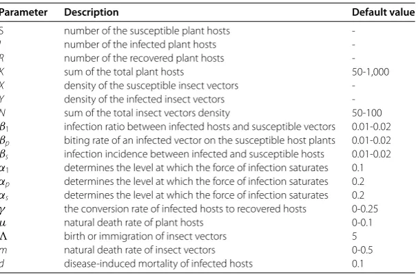
To do this, letβ= .,βp= .,βs= .,μ= .,γ = .,K= ,,= ,

α= .,αp= .,αs= .,m= .,d= ., then by a simple calculation we haveR=

. < . It follows from Figure  that the disease-free equilibrium of system () is globally asymptotically stable.

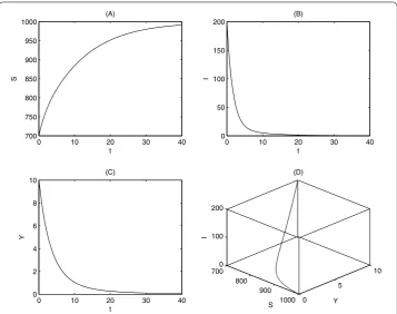
If we fixed all parameter values as follows:β= .,βp= .,βs= .,μ= .,γ = ., K= ,,= ,α= .,αp= .,αs= .,m= .,d= ., thenR= . > . For

this parameter set Figure  indicates that the endemic equilibrium of system () is globally asymptotically stable.

4.2 Discussion

Figure 1 Stability of disease-free equilibrium.The parameters are fixed as follows:β1= 0.0025,

βp= 0.0025,βs= 0.0001,α1= 0.1,αp= 0.2,αs= 0.2,μ= 0.1,γ= 0.4,K= 1,000,= 5,m= 0.3,d= 0.1, and

the initial values are (S0,I0,Y0) = (700, 200, 10). The time series charts forS(t),I(t),Y(t) and the phase diagram

are given in (A), (B), (C), and (D), respectively.

in Section . In detail, the existence, local stability, and global stability of the disease-free equilibrium and endemic equilibrium are investigated in Section . By employing a suit-able Lyapunov function, and the second additive compound matrix method, the main re-sults as shown in Theorems . and . have been derived. Our main rere-sults indicate that ifR≤, then the disease-free equilibrium is globally asymptotically stable in, and the unique endemic equilibrium is globally asymptotically stable provided thatR> . It fol-lows from these results that the basic reproduction numberRplays an important role in

determining the persistence or dying out of the disease.

Note that the basic reproduction number,R, is a strictly increasing function with re-spect to the parametersβ,βp,βs, whereas it decreases the function with respect to

pa-rametersm, ω. The parametersα,αp,αshave no relations to the value ofR. That is,

the total number of the host plant, birth rate of the vector, and incidence rate of the dis-ease can positively affect the value ofR; while the death rate of the host plant, the death rate of the vector, and the disease-induced death rate can negatively affect the value of

R; but the saturation rate of the incidence has no relation to the value ofR. Those

re-sults are useful and could help us to design optimal control strategies for disease control. For example, if under natural conditions the value ofRis greater than , then it follows from Theorem . that the endemic equilibrium is globally stable. This means that the disease will be an endemic. However, we can take measures to reduce the values of in-cidence rateβ,βp, and (or)βs, such that the value ofRcan be reduced until it is less

Figure 2 Stability of endemic equilibrium.The parameters are fixed as follows:β1= 0.01,βp= 0.02, βs= 0.01,α1= 0.1,αp= 0.2,αs= 0.2,μ= 0.1,γ= 0.4,K= 1,000,= 5,m= 0.3,d= 0.1, and the initial values

are (S0,I0,Y0) = (700, 200, 10). The time series charts forS(t),I(t),Y(t), and the phase diagram are given in (A), (B),

(C), and (D), respectively.

Competing interests

The authors declare that they have no competing interests.

Authors’ contributions

Each of the authors, RS, HZ and ST, contributed to each part of this work equally and read and approved the final version of the manuscript.

Acknowledgements

The first author is supported by Postdoctoral Science Foundation of China (no. 2011M501428) and Young Science Funds of Shanxi (no. 2013021002-2). The third author is supported by National Natural Science Foundation of China (11171199). The authors would like to thank the anonymous reviewers for their helpful comments, which improved the quality of this paper greatly.

Received: 20 December 2013 Accepted: 21 January 2014 Published:07 Feb 2014 References

1. Liang, X, Ru, R, Wu, Y, Peng, X: Research progress of vector-borne plant disease. Biol. Eng. Prog.21, 11-17 (2001) 2. Gilligan, CA: An epidemiological framework for disease management. Adv. Bot. Res.38, 1-64 (2002)

3. Gilligan, CA: Sustainable agriculture and plant disease: an epidemiological perspective. Philos. Trans. R. Soc. Lond. B, Biol. Sci.363, 741-759 (2008)

4. Jeger, MJ, Madden, LV, van den Bosch, F: The effect of transmission route on plant virus epidemic development and disease control. J. Theor. Biol.258, 198-207 (2009)

5. Jeger, MJ, van den Bosch, F, Madden, LV: Modeling virus- and host-limitation in vectored plant disease epidemics. Virus Res.159, 215-222 (2011)

6. Madden, LV, Jeger, MJ, van den Bosch, F: A theoretical assessment of the effects of vector-virus transmission mechanism on plant virus disease epidemics. Phytopathology90, 576-594 (2000)

7. Grilli, MP, Holt, J: Vector feeding period variability in epidemiological models of persistent plant viruses. Ecol. Model. 126, 49-57 (2000)

8. Jeger, MJ, Holt, J, van den Bosch, F, Madden, LV: Epidemiology of insect-transmitted plant viruses: modelling disease dynamics and control interventions. Physiol. Entomol.29, 291-304 (2004)

10. McCormack, RK, Allen, LJS: Disease emergence in deterministic and stochastic models for host and pathogen. Appl. Math. Comput.168, 1281-1305 (2005)

11. Madden, LV: Botanical epidemiology: some key advances and its continuing role in disease management. Eur. J. Plant Pathol.115, 3-23 (2006)

12. Meng, XZ, Li, ZQ, Wang, XL: Dynamics of a novel nonlinear SIR model with double epidemic hypothesis and impulsive effects. Nonlinear Dyn.59, 503-513 (2010)

13. Meng, XZ, Li, ZQ: The dynamics of plant disease models with continuous and impulsive cultural control strategies. J. Theor. Biol.266, 29-40 (2010)

14. Cai, L, Li, X: Global analysis of a vector-host epidemic model with nonlinear incidences. Appl. Math. Comput.217, 3531-3541 (2010)

15. Cunniffe, NJ, Gilligan, CA: Invasion, persistence and control in epidemic models for plant pathogens: the effect of host demography. J. R. Soc. Interface44, 439-451 (2010)

16. Muldowney, JS: Compound matrices and ordinary differential equations. Rocky Mt. J. Math.20, 857-872 (1990) 17. van den Driessche, P, Watmough, J: Reproduction numbers and sub-threshold endemic equilibria for compartmental

models of disease transmission. Math. Biosci.180, 29-48 (2002)

18. Arino, J, McCluskey, CC, van den Driessche, P: Global results for an epidemic model with vaccination that exhibits backward bifurcation. SIAM J. Appl. Math.64, 260-276 (2003)

19. LaSalle, JP: The Stability of Dynamical Systems. SIAM, Philadelphia (1976)

20. Fonda, A: Uniformly persistent semidynamical systems. Proc. Am. Math. Soc.104, 111-116 (1988)

21. Smith, HL, Thieme, H: Convergence for strongly order-preserving semiflows. SIAM J. Math. Anal.22, 1081-1101 (1991) 22. Smith, HL: System of ordinary differential equations which generate an order preserving flow. A survey of results.

SIAM Rev.30, 87-113 (1988)

23. Hirsch, MW: System of differential equations which are competitive or cooperative, IV. SIAM J. Math. Anal.1, 51-71 (1988)

24. Ma, Z, Zhou, Y, Wang, W, Jin, Z: Mathematical Models and Dynamics of Infectious Diseases. China sci. press, Beijing (2004) (in Chinese)

25. Tang, S, Chen, L: Global qualitative analysis for a ratio-dependent predator-prey model with delay. J. Math. Anal. Appl. 266, 401-419 (2002)

26. Li, MY, Muldowney, JS: Global stability for the SEIR model in epidemiology. Math. Biosci.125, 155-164 (1995) 27. Zhang, J, Ma, Z: Global dynamics of an SEIR epidemic model with saturating contact rate. Math. Biosci.185, 15-32

(2003)

10.1186/1687-1847-2014-59