Comparison Of Two Different Proposed Feature Vectors For Classification Of Complex Image

(1)

Jurnal Teknologi, 42(D) Jun. 2005: 65–82 © Universiti Teknologi Malaysia

1&2

Faculty of Computer Science & Information Systems, Universiti Teknologi Malaysia, 81310 Skudai, Johor, Malaysia.

Email1: [email protected], Email2: [email protected]

COMPARISON OF TWO DIFFERENT PROPOSED FEATURE VECTORS FOR CLASSIFICATION OF COMPLEX IMAGE

MUHAMMAD FAISAL ZAFAR1 & DZULKIFLI MOHAMAD2

Abstract. Many applications of pattern recognition use a set of local features for recognition purpose. Instead of using only local features, this paper presents a method to extract features from image body globally as well. The system takes into account several geometrical effects such as area, Euclidean distance etc and their different ratios. It utilizes thresholding and region extraction methods for gray level trademarks images, which furnish these images and segment their separate portions. Thus both local and global traits are constructed that take advantage of the pixel statistics to form a more compact representation of the image, while maintaining good recognition accuracies. Two feature vectors have been proposed. These feature vectors are comprised of nine and seven constituents, respectively. Formation of individual features is very simple involving uncomplicated ratios of geometric and numeric estimate of images’ pixels. The vectors designed are based on the invariance properties of individual features. One feature vector is invariant to rotation, translation and size, while the other has an extra invariance regarding scale. In addition, a comparative study on two feature sets is described using backpropagation neural network (BPN) as a classifier. The classification results are encouraging which ranges from 74 to 94% for different data sets.

Keywords: Pattern recognition, trademark matching, feature extraction, segmentation, backpropa-gation neural network

1.0 INTRODUCTION

The essential step to recognize an object is to define the descriptions of the object and then extract the features. There are many different methods to represent 2-D images such as boundary, topological, shape grammar, description of similarity etc. [1-3]. However, there is no algorithm which shows how to select the representation or choose the features [2]. In general, the selection of descriptors will be dependent on the applications in hand as well as the experience of the user. Features should be chosen so that they are insensitive to noise-like variation in the pattern and keep the number of features small for easy computation [4].

(2)

no colours and texture in binary images and these features are, therefore, unlikely to be useful [8].

Shape-based image matching, however, can be applied in the case of binary images. Shape representation is usually required to be invariant to geometric transformations such as translation, rotation, and scaling [9]. Methods of shape representation can be divided into two categories: boundary based and region based [5, 6]. The methods in the first category utilize the entire shape region. Boundary-based methods include Fourier descriptors [10, 11] and polygonal approximation [12]. Most boundary-based features such as Fourier descriptors require that the boundary of the shape is closed in order to be rotation invariant [8]. Moment invariants are commonly used region-based shape features [13], so they apply mainly to images with solid objects of filled regions. Many applications of pattern recognition use a set of local features for recognition purpose. This paper presents a method to extract features from image body globally as well. The system takes into account several geometrical effects such as area, Euclidean distance etc, and their different ratios. It utilizes thresholding and region extraction methods for gray level trademarks images, which furnish these images and segment their separate portions. Thus both local and global traits are constructed that take advantage of the pixel statistics to form a more compact representation of the image, while maintaining good recognition accuracies. Two feature vectors have been proposed. These feature vectors are comprised of nine and seven constituents respectively. Formation of individual features is very simple involving uncomplicated ratios of geometric and numeric estimate of images’ pixels. The vectors designed are based on the invariance properties of individual features. One feature vector is invariant to rotation, translation and size, while the other has an extra invariance regarding scale.

2.0 TRADE MARK RECOGNITION/MATCHING

A trademark is a combination of many representations, thus, it deserves a great attention in pattern recognition. Basically, trademark identification falls into the category of two dimensional objects (2-D) representation of computer vision. In a 2-D scene, the object is measured in two-space co-ordinates. Thus, its subject is grouped under 2-D object recognition system [14].

(3)

transformations such as translation, scaling, and rotation. However, the main weakness of model-based methods is their big dependency on the defined model and its placement [17]. In boundary-based methods, edge detection normally leads to incomplete description of the image, i.e. edges do not build closed boundaries of the homogeneous image regions, thus do not lead to a complete partitioning. This is due to the fact that the image noise edges are broken or do not represent the boundaries of the regions (spurious edges). An error in a symbolic description can be either quantitative (an edge is not as long as expected) or qualitative (an edge is missing or unwanted) [18]. Both these problems can be avoided by using region based method [19].

As regards to the choice of classifier, it is now established that multilayered neural networks are able to match, and often improve upon, the performance of conventional classifiers [20, 21]. They do not need any mathematical model to determine the system output depending on the given inputs. Instead, they behave as model free estimators and their output is the closest to the already “learned” patterns [22]. They have conventionally been used for a variety of automatic target detection, character recognition, face recognition and control etc. [23-27], but in case of multiple integrated object matching such as trademark, these are yet to be found. It was therefore decided to carry out work to assess the usefulness of neural network technique such as backpropagation neural network (BPN). BPN is typically proposed as a powerful tool, capable of solving complex mapping problem.

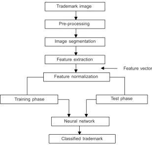
As the task is concerned with techniques for three major classes, i.e. image segmentation, recognition and interpretation, we have achieved segmentation [28] by using connected component algorithm [29], image recognition using BPN [20] and image interpretation by feeding results from BPN model to an exiting image data base. The entire exercise was done with an eventual aim of developing an efficient matching model for trademarks. The block diagram of the proposed system is shown in Figure 1.

3.0 PRE-PROCESSING

A digitized image of trademark is acquired by a scanner. To present this image for classification purpose, it is processed by applying thresholding and segmentation techniques.

3.1 Image Thresholding

(4)

automatically selected by the system [30]. Therefore, automatic thresholding has been applied. It analyzes the gray value distribution in an image by using a histogram of the gray values, to select the most appropriate threshold. The threshold is chosen using the algorithm [30] shown in Figure 2:

Figure 1 Block diagram of the system

Trademark image

Feature normalization Pre-processing

Test phase Training phase

Feature extraction

Feature vector Image segmentation

Classified trademark Neural network

Figure 2 Iterative threshold selection

(i) Select an initial estimate of the threshold, T. A good initial value is the average

intensity of the image.

(ii) Partition the image into two regions, R1 and R2, using the threshold T.

(iii) Calculate the mean gray values µ₁ and µ₂ of the partitions R₁ and R₂.

(iv) Select a new threshold:

T = (µ1 + µ2) / 2

(v) Repeat steps 2-4 until the mean values µ₁ and µ₂ in successive iterations do not

(5)

3.2 Image Segmentation

Segmentation is applied for region extraction. It is the process of grouping pixels to regions according to proximity (connectivity) and similarity (homogeneity). The large amount of region extraction methods can be classified in several ways. One possibility is to separate the regions by similarity and connectivity evaluation. This is done independently from the image raster by storing all pixels properties in a so-called measurement space (e.g. a histogram). Then, the definition of the classes can be used to classify the pixels: each pixel is labeled with the identity number of the class. In the second step, pixels of the same class which are also connected in the image space are grouped to homogeneous regions. It performs the proximity criterion, which can be

easily done by connected-components algorithms. A segmentation of an image f(x, y)

is a partition of f(x, y) into sub images R₁, R₂, …, R_n such that the following constraints

are satisfied [31]:

•

n i i

R R

=

1

∪

• R_i is a connected region, i = 1, 2, …, n.

• Ri ∩Rj =φ, i ≠ j

• P(R_i) = TRUE for i = 1, 2, …, n.

• P(R_i_{U. R}_i) = FALSE for i≠j.

Here P(R_i) is a logical predicate defined over points in set R_i and Ø in the null set.

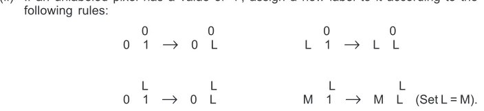
Figure 3 shows a sequential algorithm for finding connected components in an image. This algorithm is a two-pass algorithm, which labels the regions according to specific patterns (see Figure 3). The first pass scans the binary image and assigns any unlabeled

(i) Scan the binary image left to right, top to bottom.

(ii) If an unlabeled pixel has a value of '1', assign a new label to it according to the following rules:

0 0 0 0

0 1 → 0 L L 1 → L L

L L L L

0 1 → 0 L M 1 → M L (Set L = M).

(iii) Determine equivalence classes of labels.

(iv) In the second pass, assign the same label to all elements in an equivalence class.

(6)

pixel, a new label. In the assignment of these labels, the labels of neighboring pixels are considered. During the second pass, the labels of pixels are changed to the labels of their equivalence class.

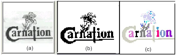
Figure 4 shows the result of automatic thresholding (Figure 4b) and component labeling (Figure 4c).

Figure 4 Component labeling: (a) A logo containing connected components, (b) Result of automatic thresholding, (c) Result of component labeling

(a) (b) (c)

4.0 FEATURE EXTRACTION

Pattern recognition in image processing requires the extraction of features from regions of the image, and the processing of these features with a pattern recognition algorithm. We consider the feature extraction part of this processing with a focus on the problem of trademark matching in pattern recognition.

4.1 Image Investigation

Many of the features used in applications such as this tend to be local in nature, which means their calculation requires a connected region of the image over which, an average or other statistic is extracted. Once the scene is segmented into regions, we can determine the geometrical properties of regions which can be used in the matching /

recognition process. We assume that each region is represented by a l ×m binary

image b(x, y) where l and m are representing height and width respectively. Then, area

or size ‘a’ of the region is a total number of pixels occupied by the region [29]. It is

given by:

( )

m n

i

x y

a b x , y i , , ,r

= =

=

∑ ∑

=

0 0

1 2… ₍₁₎

The total image area, ‘A’, will be sum of all the regions and given by:

r i i

A a

=

∑

1

(7)

Here, image means the area of interest in the scene excluding background, so

background pixels, ‘B’, are given by:

( )

(

)

B= f x , y −A (3)

Sum of differences, ‘S’, of every region area to the total image area is calculated as:

(

)

r

j j

S A a

=

∑

−

1

(4)

Euclidean distance (termed Minkoski metric) of all the regions from origin (0,0) is given by:

/ r

i i

d a

=

 

=  



∑



1 2 2 1 2

1

(5)

Euclidean distance of the three biggest regions of the image from origin (0,0) is given by:

/ r i i

d a₋

=

 

=  



∑



1 2 2

2 2 2

0

(6)

4.2 Feature Formation

Making use of the above mentioned properties, the following features (ratios) have been proposed:

Ratio of Euclidean distance of all the regions areas to total image area, i.e. from Equations (2) and (5):

d r

A

= 1

1 (7)

Ratio of Euclidean distance of three biggest regions’ areas to total image area, i.e. from Equations (2) and (6):

d r

A

= 2

2 (8)

Ratio of total image area to sum of differences of all regional areas and image area, i.e. from Equations (2) and (4):

A r

S

=

(8)

Ratio of sum of total image area and total number of regions to greatest segment area. i.e.

r A r r

a

+ =

4 (10)

Ratio of greatest segment area to the total image area, i.e.

r a r

A

=

5 (11)

Ratio of second greatest segment area to the total image area, i.e.

r a r

A

−

= 1

6 (12)

Ratio of third greatest segment area to the total image area, i.e.

r a r

A

−

= 2

7 (13)

Ratio of background pixels to total image area, i.e. from Equations (2) and (3):

B r

A

=

8 (14)

Ratio of background pixels minus image area to background pixels plus image area. i.e. from Equations (2) and (3):

B A

r

B A

− =

+

9 (15)

4.3 Feature Vectors

Two features vectors, V₁ and V₂, are designed based of the invariance properties of

the above proposed features. V₁ is invariant to rotation, translation and size, while V₂

has an extra invariance regarding scale.

{

}

{

}

V r ,r ,r ,r ,r ,r ,r ,r ,r

V r ,r ,r ,r ,r ,r ,r

= =

1 1 2 3 4 5 6 7 8 9

2 1 2 3 4 5 6 7

5.0 CLASSIFICATION

(9)

techniques in this area which has been used in this work for classification and recognition purposes.

5.1 Backpropagation Neural Network

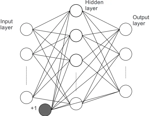
Figure 5 shows a BPN network with an input layer, one hidden layer and an output layer. In such an architecture, information is processed as follows: the outputs from the processing element (PEs) of the input layer, after multiplying with the corresponding interconnecting weights, serve as inputs to the PEs of the hidden layer. The outputs from the PEs of the hidden layer, after multiplication with corresponding interconnecting weights, serve as input to the PEs of the output layer. A bias processing element supplies a constant output of +1 to all the PEs of the hidden and output layer. BPN models with more than one hidden layer, process information on the same principle.

Figure 5 A typical BPN with one hidden layer

Input layer

+1

Output layer Hidden

layer

For a PE, the output is typically a function of the sum of input into it. For BPN models, PEs with linear, sigmoid and hyperbolic tangent transfer function are typically used depending on the position of the PE in the network architecture and the nature of the problem under consideration. With sigmoid PEs in the hidden and output layer, the output of a PE in the network’s output layer becomes highly non-linear function of the input to the network. For only one PE in the output layer, the network can be

thought of as representing a non-linear function of the inputs. For n PEs in the input

layer and m in the output layer, the network represents m non-linear functions of n

(10)

5.2 Sample Preparation

We first test the matching accuracy of the proposed methods using the different patterns of every image, as shown in Figure 7. Three small databases of thirty, forty, and fifty logos, scanned as gray images having size from 100 by 100 pixels to 120 by 120 pixels using resolution 200 dpi, were generated by rotating these images by 90, 13, and 180 degrees clockwise. Then, these were converted into binary form by applying automatic thresholding. In Figure 7, the original image is denoted as image a, and its rotated versions as images b, c, and d.

Figure 6 BPN Algorithm

Start

Exceeded max. iteration? Intialize random weights

Get next training vector

End of epoch?

Error within tolerance? Backward pass (Adapt weight using back -propagation difference equation)

Foward pass

(Run network to obtain output layer values

Yes

Declare success save training

weight

Declare failure network did not converge within

iteration limit

End No

(11)

5.3 Feature Normalization

Feature normalization is normally performed to rescale the data to a required range and it is done before matching (training and recognition) process. As BPN has been used as matching technique that uses the uni-polar sigmoid function, it requires the training and testing data to be in the range of [0, 1]. Sometimes the feature’s output is out of range [0, 1], thus the linear scaling to unit variance technique has been used. The formula for this is [33]:

x l x

u l

− =

−

where l and u are lower and upper bounds respectively for feature component x.

5.4 Training Phase

In the BPN models, sigmoid PEs were used in the hidden and output layer. Thirty-four, forty, and fifty output layer PEs corresponded to thirty-Thirty-four, forty, and fifty logos to be recognized. For example, a ‘high’ output value on the first PE in the output layer and ‘low’ on the others would mean that the network classifies the input as a logo 1. As another example, a network output vector of [0.00 0.01 0.16 0.02 0.09 0.96 0.13 0.00 --- 0.15 0.04] would be translated as the model classifying the input image as logo 6.

Experiments were started with a strict convergence criterion: training was stopped only when the network classified all the training samples correctly. While checking

the network’s performance during training, an output layer PE’s output value of ≥ 0.9

was translated as ‘high’. Thus, for this criterion, an output vector [0.00 0.03 0.06 0.12 0.09 0.16 0.03 0.91 0.17 --- 0.15 0.14] for logo 8 in the training sample set would be termed as proper classification; a 0.85 instead of 0.91 in the output vector would render the training input as not properly recognizable till that stage in the training process. Table 1 shows the summary of different parameters values used for BPN during training phase.

Figure 7 Different patterns of a trademark image

(c) (d)

(12)

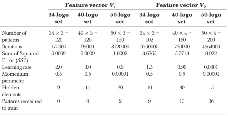
Table 1 Details of different parameter values used for BPN during training phase

Feature vector V₁ Feature vector V₂ 34-logo 40-logo 50-logo 34-logo 40-logo 50-logo

set set set set set set

Number of 34 × 3 = 40 × 3 = 50 × 3 = 34 × 3 = 40 × 4 = 50 × 4 =

patterns 120 120 150 102 160 200

Iterations 175000 95000 3120000 9790000 730000 4964000 Sum of Squared 0.0009 0.0009 1.0002 3.6365 5.7713 8.922 Error (SSE)

Learning rate 2.0 3.0 0.9 1.5 0.99 0.0001

Momentum 0.5 0.5 0.00001 0.5 0.5 0.00001

parameter

Hidden 9 11 30 10 30 15

elements

Patterns remained 0 0 2 9 13 36

to train

5.5 Testing Phase

BPN models were evaluated on samples which were not used in the initial process of setting up the training data set. This was done keeping in view the eventual aim of developing an efficient recognition / matching model, the quality of which related to translate images irrespective of size, translation, rotation, and scaling etc. Three different sets of images were being experimented; one with 34, 40, and 50 images having three different samples each. Furthermore, the performances were evaluated with respect to size separately. Tables 2 to 7 present the statistics. CRs, MRs, FRs, and RFs are abbreviation for Correct Recognitions, Multiple Recognitions, False Recognitions,

Table 2 Performance of BPN Models for vector V1 with different criteria of interpreting model output for test images smaller than reference images

Test images smaller than reference images for V1

34-images set 40-images set 50-images set

Thres- Thres- Thres- Thres- Thres- Thres- Thres-

Thres-hold 0.9 Thres-hold 0.5 hold hold 0.9 hold 0.5 hold hold 0.9 hold 0.5 hold

none none none

CRs 85.5 % 88% 88% 80% 80% 85% 84% 86% 88%

MRs 0% 3% 3% 2.5% 2.5% 5% 0% 0% 3%

FRs 8.5% 9% 9% 10% 12.5% 10% 12% 12% 9%

(13)

Table 4 Performance of BPN Models for vector V1 with different criteria of interpreting model output for

multiple size test images

Overall Test Images for V₁

CRs 91.2 % 94% 94% 87.5% 87.5% 90% 86% 86% 88%

MRs 0% 1.6% 1.6% 1.25% 1.25% 2.5% 0% 1% 3%

FRs 4.4% 4.4% 4.4% 7.5% 8.5% 7.5% 10% 11% 9%

RFs 4.4% 0% 0% 3.75% 2.75% 0% 4% 2% 0%

Table 3 Performance of BPN Model for vector V₁ with different criteria of interpreting model output for test images comparable with reference images

Test images comparable with reference images for V1

CRs 97 % 99.6% 99.6% 95% 95% 95% 88% 88% 88%

MRs 0% 0.2% 0.2% 0% 0% 0% 0% 2% 2%

FRs 0% 0.2% 0.2% 5% 4.5% 5% 8% 10% 10%

RFs 3% 0% 0% 0% 0.5% 0% 4% 0% 0%

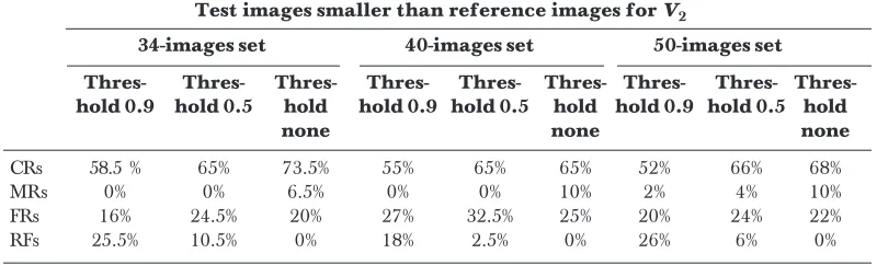
Table 5 Performance of BPN Models for vector V2 with different criteria of interpreting model output for test

images smaller than reference images

Test images smaller than reference images for V2

CRs 58.5 % 65% 73.5% 55% 65% 65% 52% 66% 68%

MRs 0% 0% 6.5% 0% 0% 10% 2% 4% 10%

FRs 16% 24.5% 20% 27% 32.5% 25% 20% 24% 22%

(14)

and Recognition Failures respectively. Three different criteria of interpreting model output, i.e. high thresholds 0.9, 0.5, 0.0, have been used.

5.6 Analysis of Performance

Although BPN models were trained on images having sizes 100 × 100 and 120 × 120

and orientations 0, 90 clock wise (cw), and 180 cw degrees but these were tested for

sizes 80 × 80 and 110 × 110 with orientations 0, 45 cw, and 90 ccw (counter clock wise).

In this way, about 800 images were tested with three sets of images for vectors V₁ and

V₂, separately. The graphical representations of performance statistics presented in

Tables 2 to 7 are shown in Figures 8 and 9.

Correct recognitions (CRs) for all the sets were from 86 to 94% under different

criteria of interpretation of model output for feature vector V₁. 34-image set showed

even greater efficiency as it had relatively smaller domain to compete. In case of feature

vector V₂, the performance for CRs was recorded from 78 to 62% under different

Table 6 Performance of BPN Model for vector V2 with different criteria of interpreting model output for

comparable with reference images

Test images comparable with reference images for V2

CRs 72 % 75% 86% 78% 80% 87.5% 72% 86% 90%

MRs 0% 0% 0% 0% 2.5% 7.5% 2% 2% 2%

FRs 14% 15% 14% 5% 5% 5% 4% 4% 8%

RFs 14% 10% 0% 17% 12.5% 0% 22% 8% 0%

Table 7 Performance of BPN Models for vector V2 with different criteria of interpreting model output for

multiple size test images

Overall Test Images for V₂

CRs 65 % 71% 74% 67.5% 74% 78% 62% 76% 78%

MRs 0% 0% 3% 4% 4% 10% 2% 4% 6%

FRs 15% 20% 23% 7.5% 10% 12% 13% 16% 16%

(15)

Figure 8 (a), (b), and (c) are the graphical representations of performance of BPN models for large, small and average of both type of images respectively for vector V1. (d), (e), and (f) are the similar

CRs

RFs 0.9

FRs

MRs

0 0.5 0 0.5 0.9 0 0.5 0.9

100%

0% 50%

34-Image set 40-Image set 50-Image set

(a)

0.9

0 0.5 0 0.5 0.9 0 0.5 0.9 100%

0% 50%

34-Image set 40-Image set 50-Image set CRs RFs FRs MRs (b) 88% 86% 86% 90% 87.50% 87.50% 94% 94% 91.20% 3% 1% 0% 2.50% 1.25% 1.25% 1.60% 1.60% 0% 9% 11% 10% 7.50% 8.50% 7.50% 4.40% 4.40% 4.40% 0% 2% 4% 0% 2.75% 3.75% 0% 0% 4.40% CRs RFs 0.9 FRs MRs

0 0.5 0 0.5 0.9 0 0.5 0.9

100%

0% 80%

34-Image set 40-Image set 50-Image set

60% 40% 20% (c) 68% 66% 52% 65% 65% 55% 73.50% 65% 58.50% 10% 4% 2% 10% 0% 0% 6% 0% 0% 22% 24% 20% 25% 32.50% 27% 20% 24.50% 16% 0% 6% 26% 0% 2.50% 18% 0% 10.50% 24.50%

0 0.5 0.9 0 0.5 0.9 0 0.5 0.9

50-Image set 40-Image set 34-Image set 90% 86% 72% 87.50% 80% 78% 86% 75% 72% 2% 2% 2% 7.50% 2.50% 0% 0% 0% 0% 8% 4% 4% 5% 5% 5% 14% 15% 14% 0% 8% 22% 0% 12.50% 17% 0% 10% 14% 0% 10% 20% 30% 40% 50% 60% 70% 80% 90%

0 0.5 0.9 0 0.5 0.9 0 0.5 0.9

50-Image set 40-Image set 34-Image set CRs MRs FRs RFs 80% 0% 40% 30% 20% 50% 60% 70%

0 0.5 0.9 0 0.5 0.9 0 0.5 0.9 34-Image set 40-Image set 50-Image set CRs RFs FRs MRs 80% 0% 40% 20% 60%

0 0.5 0.9 0 0.5 0.9 0 0.5 0.9 34-Image set 40-Image set 50-Image set CRs RFs FRs MRs 100% (e) (d) 78% 76% 62% 78% 74% 67.50% 74% 71% 65% 6% 3% 2% 10% 4% 4% 3% 0% 0% 16% 16% 13% 12% 10% 7.50% 20% 20% 15% 0% 4% 23% 0% 12% 21% 0% 10% 20% 80% 0% 40% 20% 60%

0 0.5 0.9 0 0.5 0.9 0 0.5 0.9

(16)

criteria of interpretation of model performance. It means reduction of features has significant effect on the performance of the model along with scaling factor, but interestingly recognition performance increases with bigger image sets, i.e. for 40 and 50 image sets.

Multiple recognitions (MRs) mean that there are more than one output for a test image as some images have very close and quite similar features.The chances of MRs and FRs increase with an increase in logos; has been observed in case of feature

vector V₁,and it is quite understandable because the model has more images to compare

with. However, FRs were minimum under feature vector V₂ set and performance of

the model for CRs was also improved with an increase in sample logos.

Another interesting factor was observed that the performance of models, both for

feature vector V₁ and feature vector V₂, was excellent for test images equal or greater

scale and size than that of reference images (Tables 3 and 6), but it was badly affected for test images having smaller scale and size than that of reference images (images used in training phase) (Tables 2 and 5).

The comparison of performances between feature vector V₁ and feature vector V₂

with pragmatic interpreting criterion of 0.5 (neither too strict ‘0.9’ nor too loose ‘0.0’)

are shown in Figure 9. It is obvious from this graph that models using feature vector V₁

give better recognition rate as compared to models using feature vector V₂. In models

using feature vector V₁, the more logos are considered, the less recognition is performed.

By increasing the number of logos, it is obvious that the curve tends to be well-fitted. In this way, we are gradually losing a general behavior of the pattern concerned. At this particular point, it is found that by putting their pattern recognition features in

models using feature vector V₂, the recognition performance is improved. The fact is

depicted in models using feature vector V₂ as they have invariance to scale, size etc, to

describe one pattern behavior.

Figure 9 Performance of BPN models for both feature vectors V1 and V2 with an intermediate interpreting criterion of 0.5

76% 3% 16% 4%

74% 4% 10% 12%

71% 0% 20% 10%

86% 1% 11% 2%

87.50% 1.25% 8.50% 2.75%

94% 1.60%4.40%0%

80%

0% 20% 30% 40% 50% 60% 70%

34-Image set

40-Image set

50-Image set CRs

RFs

FRs MRs

10% 90% 100%

34-Image set

40-Image set

50-Image set

Feature vector

V1

Feature vector

(17)

6.0 CONCLUSIONS

Two feature vectors had been proposed based on global as well as local information of the image. These give more representative description of the image and therefore, allow more accurate image matching. The authors had contributed feature sets of simpler pixels ratios yet effective, in recognizing complex objects such as trademarks. These could perform robust recognition of any symbol, which is free from any imposed constraint. Since there were large number of samples to be considered, and some trademarks were very much like one another in terms of their features behavior, this had resulted in misclassification. BPN could not converge to a required value in some cases. Inadequate normalization may also be a factor as the technique used, by simply converting two of the features to 0 and 1, eliminated some useful information. The study could not focus on finding good feature normalization. However, the authors had succeeded in formulating good invariant features without undergoing a lengthy process of image normalization. The usage of the reckoning pixel information and its different ratios has several advantages. Firstly, the matching is independent of the spatial location of the regions or image contents, and therefore, the method is translation, scaling and rotation invariant by its nature.

REFERENCES

[1] Tsirikolias, K., and B. G. Mertzios. 1993. Statistical Pattern Recognition Using Efficient Two-dimensional Moments with Applications to Character Recognition. Pattern Recognition. 26(6): 877-882.

[2] Li, B. C. 1993. The Moment Calculation of Polyhedra. Pattern Recognition. 26(8): 1229-1233.

[3] Ghosal, S., and R. Mehrotra. 1993. Orthogonal Moment Operators for Subpixel Edge Detection. Pattern Recognition. 26(2): 295-306.

[4] Somaie, A. A. I. 1996. Face Identification Using Computer Vision. Ph.D. Thesis. University of Bradford. [5] Ma, W.-Y., and H. J. Zhang. 1999. Content-based Image Indexing and Retrieval. In B. Fuhrt (ed), Handbook

of Multimedia Computing. Boca Raton, FL: CRC Press. 227-254.

[6] Rui, Y. T. S., Huang, and S.-F. Chang. 1999. Image Retrieval: Current Techniques, Promising Directions and Open Issues. Journal of Visual Communications and Image Representation. 10(1): 39-62.

[7] Kankanhalli, M. S., B. M. Mehtre, and H.Y. Huang. 1999. Color and Spatial Feature for Content-based Image Retrieval. Pattern Recognition Letters. 20(1): 109-118.

[8] Fränti, P., A. Mednonogov, V. Kyrki, and H. Kälviäinen. 2000. Content-based Matching of Line-drawing Images Using the Hough Transform. International Journal on Document Analysis and Recognition IJDAR. 3: 117-124.

[9] Mehrotra, R., and J. E. Gary. 1995. Similar-shape Retrieval in Shape Data Management. Computer. 28(9): 57-62.

[10] Kauppinen, H. T. Sepp¨anen, and M. Pietik¨ainen. 1995. An Experimental Comparison of Autoregressive and Fourier-based Descriptors in 2D Shape Classification. IEEE Transactions on Pattern Analysis and Machine Intelligence. 17(2): 201-207.

[11] Persoon, E., and K. Fu. 1977. Shape Discrimination Using Fourier Descriptors. IEEE Transactions on Systems, Man and Cybernetics. 7(3): 170-179.

[12] Arkin, E. M., L. P. Chew, D. P. Huttenlocher, K. Kedem, and J. S. B. Mitchell. 1991. An Efficiently Computable Metric for Comparing Polygonal Shapes. IEEE Transactions on Pattern Analysis and Machine Intelligence. 13(3): 209-226.

(18)

[14] Rosenfeld, A. 1992. Image Analysis and Computer Vision: 1991. CVGIP: Image Understanding1. 55(3): 349-380.

[15] Mohamad. D. 1997. The Identification of Trademark Symbols Based on Modeling Techniques. Ph.D. Thesis. Universiti Teknologi Malaysia.

[16] Mohamad D., and G. Sulong. 1996. Trademark Identification Using Eigenvector Modeling Technique. Proceeding of the IASTED International Conference. Florida, U.S.A. 69-73.

[17] Cootes, T. F., and C. J. Taylor. 2000. Statistical Models of Appearance for Computer Vision. Report on Active Shape Models and Active Appearance Models.

[18] Fuchs, C., and S. Heuel. 1998. Feature Extraction. Institute for Photogrammetry, University Bonn, Germany. [19] Crysdian. C. 2001. Region-based Digital Image Segmentation Using Pixel Caste-mark and Pixel Discrimination.

Master Thesis. Universiti Teknologi Malaysia.

[20] Jain, A. K., R. P. W. Duin, and J. Mao. 2000. Statistical Pattern Recognition: A Review. IEEE Transactions on Pattern Analysis and Machine Intelligence. 22(1): 04-37.

[21] Guyon, L., I. Poujaud, L. Personnaz, G. Dreyfus, J. Denker, and Y. Le Cun. 1990. Comparing Different Neural Network Architectures for Classifying Hand-written Digits. Proc. of the Int. Joint Conf. on Neural Networks. New York. 127-132.

[22] Hecht-Nielsen, R. 1990. Neurocomputing. Reading, MA: Addison-Wesley Publishing Company.

[23] Ahmed, S. M. et al. 1995. Experiments in Character Recognition to Develop Tools for an Optical Character Recognition System. IEEE Inc. 1st National Multi Topic Conf. Proc. NUST. Rawalpindi, Pakistan. 61-67. [24] Perantonis, S. J., and P. J. G. Lisboa. 1992. Translation, Rotation, and Scale Invariant Pattern Recognition by High-order Neural Networks and Moment Classifiers. IEEE Transactions Neural Networks. 3(2): 241-251. [25] Ho, J. K., and H. S. Yang. 1994. A Neural Network Capable of Learning and Inference for Visual Pattern

Recognition. Pattern Recognition. 27(10): 1291-1302.

[26] Shaaban, Z. M. 1996. Algorithm for Off-line Upper-case Hand-written Text Recognition and its Associated Processes. Ph.D. Thesis. Universiti Teknologi Malaysia.

[27] Ferand, R. et al. 2001. A Fast and Accurate Face Detection Based on Neural Networks. IEEE Transactions on Pattern Analysis and Machine Intelligence. 23(1).

[28] van der Heijden, F. 1994. Image Based Measurement Systems: Object Recognition and Parameter Estimation. England: John Wiley & Sons.

[29] Shah, M. 1995. Fundamentals of Computer Vision. UCF, Florida, USA.

[30] Jain, R., R. Kasturi, B. G. Schunck. 1995. Machine Vision. Singapore: McGraw-Hill Series in Computer Science.

[31] Gonzalez R. C., and R. E. Woods. 2002. Digital Image Processing (Second Edition). International Edition. New Jersey: Prentice-Hall Inc.

[32] Freeman, J. A., and D. M. Skapura. 1991. Neural Networks: Algorithms, Applications and Programming Tecniques. Addison-Wesley Publishing Company.