Measurement of Cerebral Blood Flow In Humans
Using MRI with Arterial Spin Labelling
Jonna Aleide Wiersma
UCL
Wellcome Department of Imaging Neuroscience
University College London
Submitted for the Degree of Doctor o f Philosophy
University of London
ProQ uest Number: U 642195
All rights reserved
INFORMATION TO ALL U SE R S
The quality of this reproduction is d ep en d en t upon the quality of the copy subm itted.
In the unlikely even t that the author did not sen d a com plete manuscript
and there are m issing p a g e s, th e se will be noted. Also, if material had to be rem oved, a note will indicate the deletion.
uest.
ProQ uest U 642195
Published by ProQ uest LLC(2015). Copyright of the Dissertation is held by the Author.
All rights reserved.
This work is protected against unauthorized copying under Title 17, United S ta tes C ode. Microform Edition © ProQ uest LLC.
ProQ uest LLC
789 East E isenhow er Parkway P.O. Box 1346
Science
I am but a grateful tourist enjoying the sights the perspective
charting the landscape taking pictures
life looks in my eyes and smiles
its beauty more in detail
I am humbled I fly; nothing in the universe love the buzz
4 /5 /9 9
And what is good, Phaedrus, And what is not good —
Need we ask anyone to tell us these things?
Abstract
Cerebral blood flow (CBF) is an important marker for tissue well-being and brain function.
Traditionally, CBF has been measured with invasive methods using exogenous tracers.
With the introduction of arterial spin labelling (ASL) MRI techniques, non-invasive,
quantitative CBF mapping in humans became feasible. The aim of the work described in
this thesis was to implement, optimise and validate an ASL MRI technique for measuring
CBF in humans. Furthermore, the utility of this technique for longitudinal studies was to be
evaluated.
FAIR, a pulsed ASL technique, was successfully implemented. A data acquisition
and analysis protocol was proposed after an extensive survey of acquisition and
quantification issues such as rf pulse profiles, static subtraction error, voxel partial
voluming, volunteer movement and choice of CBF quantification models.
Fitting for CSF fraction resulted in an improved goodness-of-fit when compared to
the standard fit model. It was also derived that it is necessary to analyse the magnitude of
the FAIR data to avoid erroneous results. Furthermore, it was shown that the inflow delay
has to be included in the fit model for an accurate CBF value. Two image realignment
protocols were proposed and evaluated.
The CBF measurement was validated by comparing baseline and parametric CBF
results with literature values. Finally, the technique was applied in a study of CBF, inflow
delay, BOLD signal and cerebrovascular reactivity (CR) over the course of a day. The
findings were used to propose upper limits to diurnal changes in these parameters.
The standard deviation of a CBF measurement was found to be satisfactory for
functional experiments, but not for longitudinal studies where small CBF changes are of
interest. It was argued how FAIR could be made more suitable for longitudinal studies by
applying 3D-realignment to whole brain FAIR, acquired preferably at a higher magnetic
Contents
1 Introduction__________________________________________ 1
1.1 PhD project aims _____________________________________________________ 2
1.2 Thesis summary______________________________________________________ 3
2 Magnetic Resonance Imaging___________________________ 5
2.1 Magnetic resonance: microscopic description______________________________ 5
2.1.1 Chemical shift____________________________________________________ 7
2.2 Magnetic Resonance: macroscopic description_____________________________ 8
2.3 Relaxation; spin echo experiment________________________________________10
2.4 Radiofrequency pulses________________________________________________ 14
2.4.1 Slice selection; pulse simulations___________________________________ 14
2.4.2 Adiabatic pu lses_________________________________________________16
2.4.3 A standard imaging experiment____________________________________23
2.4.4 K-space________________________________________________________26
2.4.5 Echo Planar Imaging_____________________________________________28
2.5 Image weighting_____________________________________________________ 32
2.5.1 Proton density, Ti, T2 and T2* weighting_____________________________32
2.5.2 Perfusion_______________________________________________________ 33
3 Introduction to ASL Methods and BOLD fM R I_____________39
3 .1 Arterial spin labelling_________________________________________________ 39
3.1.1 Continuous ASL m ethods__________________________________________39
3.1.2 Pulsed ASL methods______________________________________________45
3.3.1 Static subtraction error, transit time, fresh inflow, Q U IPSS_____________49
3.1.3 Intravascular signal______________________________________________52
3.2 BOLD fM RI________________________________________________________ 53
4 Optimising inversion and readout puises________________ 56
4.1 Introduction_________________________________________________________56
4.2 Inversion pulses at low p o w e r__________________________________________ 57
4.2.1 M ethods_______________________________________________________ 57
4.2.2 Results and Discussion____________________________________________5 7
4.2.3 Conclusions low power inversion pulse sim ulations____________________62
4.3 Pulse profiles and interactions of inversion and readout pulses at normal power _ 62
4.3.1 M ethods_______________________________________________________ 62
4.3.2 Results and Discussion____________________________________________65
4.3.3 Conclusions regarding pulse profile interactions_______________________71
5
Measuring CBF with FAIR_____________________________ 72
5.1 Introduction_________________________________________________________72
5.2 FAIR pulse sequence implementation____________________________________72
5.3 A basic CBF quantification experiment___________________________________78
5.3.1 Data acquisition_________________________________________________78
5.3.2 Modelling the d a ta_______________________________________________82
5.4 Quantification issues__________________________________________________ 99
5.4.1 Partial voluming_________________________________________________99
5.4.2 Macrovascular contributions: flow spoiling__________________________113
5.4.3 The static subtraction erro r_______________________________________116
5.4.4 Model selection_________________________________________________119
5.4.5 Optimising the time efficiency o f the CBF measurement________________133
5.4.6 Volunteer Motion; Realignment____________________________________137
6
In vivo results: baseline and hypercapnie CBF and Inflow
delay In man__________________________________________ 150
6.1 Introduction________________________________________________________ 150
6.2 A parametric hypercapnia experiment___________________________________ 150
6.2.1 Materials and Methods___________________________________________150
6.2.2 Results and discussion___________________________________________153
6.3 Variability o f CBF and inflow delay over 11 volunteers____________________ 166
6.3.3 Materials and Methods___________________________________________166
6.3.4 Results and discussion___________________________________________167
7
CBF, Inflow delay, BOLD signal and cerebrovascular
reactivity over the course of a day________________________ 174
7.1 Introduction________________________________________________________174
7.2 Inter-session movement e ffec ts________________________________________ 175
7.2.1 Minimising intersession movement_________________________________175
7.2.2 The effects out-of-plane motion; choice o f masks______________________177
7.3 Measuring CBF, inflow delay, BOLD signal and CR over the course of a day 180
7.3.1 Materials and methods___________________________________________180
7.3.2 Results_________________________________________________________183
7.3.3 Discussion______________________________________________________197
7.4 Appendices_________________________________________________________ 199
8
Discussion and Conclusions_________________________ 212
8.1 The implementation and optimisation of quantitative CBF measurements_____ 212
8.2 Future W ork________________________________________________________216
List of Figures
Figure 2-1 Two dipoles A and X within a molecule. The field at spin A due to the spin X
depends on the angle 0 and the distance r between the dipoles (adapted from Gadian,
1995)...11
Figure 2-2 The principle of adiabatic pulses...18
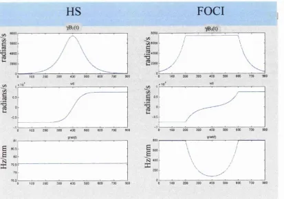
Figure 2-3 HS and FOCI pulses: rf (top) in radians/s, Aco(middle) in radians/s and
gradient shapes (Hz/mm) for HS (left) and FOCI C-shape pulse (right)...22
Figure 2-4 Simulated profiles of HS and FOCI pulses as described in the text. HS: red
line, FOCI: dark blue line, striped light blue line gives -7.5 mm, +7.5mm inversion
boundaries of a perfect pulse...22
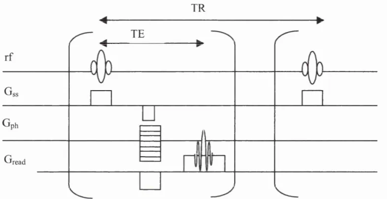
Figure 2-5 Basic MRI experiment. Gss: slice selective gradient, Gph: phase encoding
gradient, Gread: readout/frequency encoding gradient. TE: echo time, TR: repetition
time...25
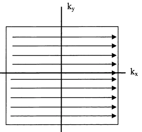
Figure 2-6 K-space sampling scheme for a FLASH sequence: one k-space line per
excitation...29
Figure 2-7 K-space sampling scheme for an EPI sequence: all k-space lines are acquired
after one excitation... 29
Figure 2-8 EPI pulse sequence...30
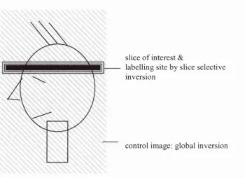
Figure 3-1 Schematic representation of basic setup continuous labelling ASL... 42
Figure 3-2 Schematic representation of basic setup FAIR, a pulsed labelling technique....48
Figure 4-1 Inversion profiles for HS pulse, )i P=3200 radians/s,...59
Figure 4-2 Inversion profiles for FOCI C-shape pulse, |x P=3200 radians/s,... 59
Figure 4-3 Inversion profiles of the different FOCI pulses compared... 60
Figure 4-4 Experimental results for the HS (black x) and FOCI C-shape (green o) rf
pulses:...61
Figure 4-5 Illustration of a simulated one-dimensional spin echo FAIR experiment... 63
Figure 4-6 Inversion profiles: HS |X=5 radians, p=1500 s '\ Time pulse = 8ms, slice
thickness = 6mm (green o). FOCI same parameters, A - 2 (red *), A=4.5 (blue +),
\0
Figure 4-7 Readout profiles: 3-lobed sine 90° (green o), 3-Iobed sine 90'
180°(yellow/pink stripe dot), 5-lobed sine 90° (red *), 5-lobed sine 90°-180° (blue
x), 5-lobed Hamming filtered sine 90° (black 0), 5-lobed Hamming filtered sine
90°-180° (magenta V). Rectangular profile (black striped line)...67
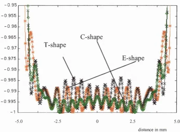
Figure 4-8 Percentage difference between SL and GL for a perfect rectangular inversion
pulse and the following readout pulses: [1-5] 3-lobed sine 90° (o), [2-5] 3-lobed sine
90°-180°(line), [3-5] 5-lobed sine 90° (*), [4-5] 5-lobed sine 90°-180° (x), [5-5] 5-
lobed Hamming filtered sine 90° (0), [6-5] 5-lobed Hamming filtered sine 90°-180°
(V). [7-5] Rectangular profile: along x-axis. Pulse profiles for the readout pulses on
their own are given in Figure 4-7... 69
Figure 4-9 Comparing the 5-lobed 90° (o) and 5-lobed 90°-180° (*) for different ratios of
inversion and effective readout slice thicknesses... 69
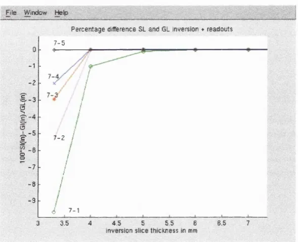
Figure 4-10 Percentage difference between SL and GL for a rectangular readout pulse of
slice thickness 3.3mm and a range of inversion pulses: [7-1] HS \i=5 radians,
p=1500 s'* , Time pulse = 8ms (o). HS FOCI same parameters, [7-2] A=2 (line),
[7-3] A=4.5 (*), [7-4] A=10 (x). [7-5] Rectangular profile (0)... 70
Figure 4-11 Profile interactions of Hamming filtered 5-lobed 90°-180° of slice thickness
3.3mm with standard HS (o), FOCI with A=2 (line), A=4.5 (*), A=10 (x) and a
perfect rectangle (0 )...70
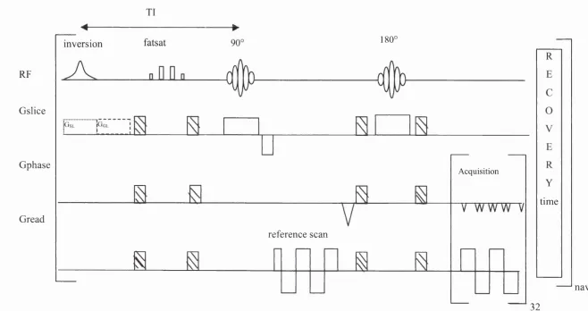
Figure 5-1 Pulse sequence for FAIR. GgL: gradient for slice selective inversion; GoL:
gradient for global inversion. The slice selective and global inversions are
alternated. Shaded pulses: spoiler gradients. RF: radiofrequency pulses. Gslice,
Gphase, and Gread: respectively slice selective gradient, phase encoding gradient,
read gradient. Fatsat: fat saturation, nav: number o f averages... 73
Figure 5-2 The normalised pulse profile of the HS pulse measured on a phantom. j l i=5
radians, p=1500 s'*; slice thickness =30 mm... 75
Figure 5-3 (a) Inversion recovery data (‘o’) and fit (‘-‘) for the FAIR slice selective
inversion for one voxel, (b) Pulse profile of 5-lobed Hamming filtered 90°-180° sine
pulses (blue); HS slice selective inversion profile (-.) and expected HS GL inversion
Figure 5-4 Static subtraction error as percentage of Mo measured on a gel phantom... 75
Figure 5-5 Slice selective (top row) and global (bottom row) inversion data over a range
o f inversion times TI... 81
Figure 5-6 FAIR (subtraction) data over a range of inversion times TI... 81
Figure 5-7 Results SL fit: (a) Inversion efficiency (Xq, (b) Tiapp in s, (c) Mq in arbitrary
units... 86
Figure 5-8 Mean SL +/- se and fit as percentage Mq - white matter voxel... 87
Figure 5-9 Mean SL +/- se and fit as percentage Mq - grey matter voxel... 87
Figure 5-10 CBF in ml/lOOg/min, without (a) and with (b) fitting for delay, (c) fitted
delay in s ... 92
Figure 5-11 Mean FAIR +/- se and CBF fit as percentage o f Mq with (a) and without (b)
delay fitted - grey matter voxel... 94
Figure 5-12 Mean FAIR +/- se and CBF fit as percentage o f Mq with (a) and without (b)
delay fitted - white matter voxel... 94
Figure 5-13 Partial voluming simulation, results grey matter with progressive CBF
partial voluming: (a) inversion efficiency, (b) Tiapp, (c) Mo, (d) CBF, (e) inflow
delay, (f) CBF from constrained analysis... 103
Figure 5-14 Partial voluming simulation, TMF model; results grey matter with
progressive CBF partial voluming ((Xo=0.99): (a) T^pp, (b) Mq, (c) fraction CSF, (d)
CBF, (e) inflow delay, (f) FAIR signal for CBF=80 ml/lOOg/min and different CSF
fractions... 106
Figure 5-15 Explaining negative FAIR signal due to CSF partial voluming; evaluation of
improved fitting models. For a grey matter voxel with a CBF of 80 ml/lOOg/min and
an inflow delay of 0.7 s with/without CSF partial voluming. (a) No CSF: dM(TI)
(black squares) overlaid on dM’(TI) (red circles), (b) Inversion recovery signal for
CSF: Mz^^(TI) (yellow striped) and Mz^^(TI) (black striped) for a CSF fraction of
25% of Mo. (c) For a 25% CSF fraction: dM’(TI) for sum of grey matter and CSF
fractions (green circles) overlaid on dM’(TI) for the grey matter fraction only (red
circles), (d) CBF and (e) inflow delay as percentage of the correct value for TMF
Figure 5-16 Grey/white matter partial voluming. Fitted parameter values for increasing
white matter fraction and for different CSF fractions. Fraction CSF=0: ITM(blue),
TMF (red); fraction CSF=0.25: ITM (green), TMF(magenta); fraction CSF=0.50:
ITM(cyan),TMF(magenta). Correct values in dashed black lines, (a) Fitted CBF,
delay of white matter is 0.7 s. (b) Fitted CBF, delay of white matter is 1.2 s. (c)
Fitted inflow delay, (input) delay of white matter is 0.7 s* (d) Fitted inflow delay,
(input) inflow delay white matter is 1.2 s * (e) Fitted Oo - not fitted in TMF model
(f) Fitted Tiapp, linear relation between grey and white matter dotted.*...112
Figure 5-17 FAIR at TI=1200ms for a range of b-values. (a) Magnitude FAIR data, (b)
Mean +/- se FAIR signal over slice (voxels at noise level not included)... 115
Figure 5-18 Simulations of the effect of the static subtraction error (SSE) on CBF and
delay values for partial volumed data. TMFo/TMFgtat’ FA IR data without/with SSE,
fitted with TM F model parameters. ITMo/ITMgtat: FAIR data without/with SSE,
fitted with ITM model parameters, (a) CBF as percentage correct value for grey
matter/CSF partial voluming. (b) delay as percentage correct value for grey
matter/CSF partial voluming (c) CBF as percentage correct value for white/grey
matter partial voluming, fraction CSF is 0. (d) delay as percentage correct value for
white/grey matter partial voluming, fraction CSF is 0... 118
Figure 5-19 Fit results for TMF (left) and ITM models (right), (a) Tiapp values in s. (b)
Mo values in arb. units. For TMF model only: (c) fitted CSF fraction (d) Voxels that
were refitted for Tiapp and Mq only (blue); nulled for display reasons within the brain
mask (red)...122
Figure 5-20 Magnitude FAIR data... 126
Figure 5-21 Results fitting magnitude FAIR data vs results standard non-magnitude
FAIR fitting. CBF in ml/lOOg/min, delay in s. (a) CBFabs, (b) CBFnon-abs, (c) delayabs,
(d) delaynon-abs, (e) Plot grey matter voxel fits, abs data (black squares), non-abs data
(red circles), abs fit (magnenta line), non-abs fit (blue line), (f) Plot white matter
voxel fits, abs data (black squares), non-abs data (red circles), abs fit (magnenta
Figure 5-22 The effect of negative FAIR signal on delay fitting in vivo: (left) for each
voxel, the longest TI value is given at which its FAIR signal is still negative; (right)
the fitted delay for FAIRnon-abs... 130
Figure 5-23 Comparing CBFO and CBFD model for fitting magnitude FAIR data with
TMF parameters... 130
Figure 5-24 Optimising dM/VTR by choice of recovery time t; TR=TI+ t; dM/VTR
given as percentage of Mq/Vs...136
Figure 5-25 Effect of out-of-plane movement on slice edges... 141
Figure 5-26 Results for optimised experiment: CBF in ml/lOOg/min (left) and delay in s
(right)... 145
Figure 5-27 Data and fit for (a) mean of grey matter mask, (b) mean of white matter
mask, (c) single white matter voxel, (d) single grey matter voxel. The mask data
have been normalised by Mo before averaging and fitting. All data have been
realigned... 149
Figure 6-1 Raw magnitude FAIR data for all PetCOi states... 154
Figure 6-2 Raw BOLD data for all PetC02 states... 154
Figure 6-3 Realignment results for BOLD data, when 3d realignment is applied over all
sessions. Translation in x, y and z and rotation around x, y and z axes... 155
Figure 6-4 CBF in ml/lOOg/min for all PetC02 states... 157
Figure 6-5 Inflow delay in s for all PetC02 states... 157
Figure 6-6 Mean CBF +/- se for global (black ^), grey matter (red o) and white matter
(green square) segments. Linear regression plotted as line... 159
Figure 6-7 Mean inflow delay +/- se for global (black ^), grey matter (red o) and white
matter (green square) segments. Linear regression plotted as line... 159
Figure 6-8 Comparing fitting with/without inflow delay: results for CBFD and CBFO
models for grey matter and global segments. For both segments the lower line is the
result of the CBFO fit... 163
Figure 6-9 Mean BOLD signal +/- se for global (black ^), grey matter (red o) and white
matter (green square) segments. Linear regression plotted as line... 165
Figure 6-10 Percentage CBF change vs percentage BOLD change for grey matter.
Figure 6-11 CBF maps for all 11 volunteers (plotted left to right, row by row)... 171
Figure 6-12 Inflow delay maps for all 11 volunteers (plotted left to right, row by row)...172
Figure 6-13 Results for a voxel with normal inflow delay (-0.5s), left, and for voxel with
shortened inflow delay ( - 0.2s), right, (a) Ti weighted structural scan of this slice.
Second row (b), (c): inflow delay maps with red cross and circle marking the voxel,
third row (d), (e): SL fit, bottom row (e), (f): fit of FAIR data. Note the scales are
not equal for corresponding plots. Taken from data of volunteer number 1... 174
Figure 7-1 Minimising inter-session movement effects with a dedicated repositioning
device...176
Figure 7-2 Realignment parameters for BOLD inter-realignment, taken as a measure for
volunteer movement over all 4 sessions. Each session consists o f 2*12 BOLD
acquisitions, one BOLD data set for the rest and one for the hypercapnia state. Red:
movement in/around z, green: movement in/around y, blue: movement in/around x.
Mind the different scales in the plots. Results for first 4 volunteers. Volunteer
M05965 - marked by an asterisk - showed such large out-of-plane shifts (i.e. in z)
that all her data were discarded. Volunteer M06004 has one session with out-of
plane shifts larger than 5 mm. Volunteer M06044 - marked with ^ - has only data
for rest states, hence only 4*12=48 BOLD acquisitions... 184
Figure 7-3 Mean +/- se CBF for all volunteers over the course of a day, standard grey
matter mask. M05808: red circles; M06004: blue diamonds; M06044: green squares;
M06094: magenta triangles; M06192: cyan pentagons, M06242: black crosses;
M06348: yellow stars...187
Figure 7-4 Mean +/- se CBF averaged over all volunteers, red circles: standard grey
matter mask; blue diamonds: 86% grey-stmc mask; green squares: global mask... 187
Figure 7-5 Mean +/- se inflow delay for all volunteers over the course of a day, standard
grey matter mask. M05808: red circles; M06004: blue diamonds; M06044: green
squares; M06094: magenta triangles; M06192: cyan pentagons, M06242: black
crosses; M06348: yellow stars... 188
Figure 7-6 Mean +/- se inflow delay averaged over all volunteers, red circles: standard
Figure 7-7 Mean +/- se BOLD for all volunteers over the course of a day, standard grey
matter mask. M05808: red circles; M06004: blue diamonds; M06044: green squares;
M06094: magenta triangles; M06192: cyan pentagons, M06242: black crosses;
M06348: yellow stars...191
Figure 7-8 Mean +/- se BOLD averaged over all volunteers, blue diamonds: 86%
grey-struc mask; green squares: global mask...191
Figure 7-9 Mean +/- se CR for all volunteers over the course of a day, standard grey
matter mask. M05808: red circles; M06004: blue diamonds; M06094: magenta
triangles; M06192: cyan pentagons, M06242: black crosses; M06348: yellow stars. 193
Figure 7-10 Mean +/- se CR averaged over all volunteers, red circles: standard grey
matter mask;... 193
Figure 7-11 Mean +/- se BOLD relative CR for all volunteers over the course of a day,
standard grey matter mask. M05808: red circles; M06004: blue diamonds; M06094:
magenta triangles; M06192: cyan pentagons, M06242: black crosses; M06348:
yellow stars... 196
Figure 7-12 Mean +/- se BOLD relative CR averaged over all volunteers, blue diamonds:
List of Tables
Table 4-1 Illustration of phase shift scheme required for simulation one-dimensional spin
echo FAIR experiment To illustrate the effect of (imperfections in) the 180°
refocussing pulse, the magnetization in x,y,z is calculated here for a perfect
inversion and 90° pulse. The effect of the required spoiler gradient is mimicked by
summing four experiments, each run with a different phase shift applied before and
after the 180° refocussing pulse. By using different phase shifts cp of 0,7T,-1/271 and
1/271 radians for the runs, the sum of the four simulations adds up to magnetizations
without any contributions of the imperfections of the refocussing pulse. This is what
is achieved in vivo by using spoiler gradients... 64
Table 4-2 Effective slice thicknesses of simulated pulses... 66
Table 5-1 Static subtraction error as percentage Mq measured on a gel phantom for a
range of inversion times TI...78
Table 5-2 Parameters for basic FAIR experiment... 78
Table 5-3 Results for grey and white matter masks: Tiapp, CBF and delay values. All
values are listed in the following format: mean +/- standard deviation (% mean);
median (% mean). For CBF values the standard error (SB) is also given. The
standard deviations on the CBF ratios were calculated using the standard errors 96
Table 5-4 Partial voluming simulation parameters. All other unmentioned simulation
settings are the same as used in the data analysis of section 5.3.2... 100
Table 5-5 Simulation parameters for white matter... 111
Table 5-6 Results Goodness-of-fit test TMF vs ITM models for SL fit : percentage
voxels in mask with Q > 0.001... 121
Table 5-7 Comparing the mean sd as percentage mean value voxel for TMF and ITM
models... 123
Table 5-8 Results goodness-of-fit test TMF vs ITM models in FAIR fit: % voxels in
mask w ith... 123
Table 5-9 CBF, delay and CBF ratios for fitted FAIR data with TMF and ITM
Table 5-10 Results goodness-of-fit test magnitude vs non-magnitude FAIR fitting, using
parameters from the TMF model: percentage voxels in mask with Q > 0.001... 125
Table 5-11 Comparing the relative errorbars -mean sd as percentage mean value voxel-
for magnitude and non-magnitude FAIR fitting of experimental data, with TMF
model inputs...125
Table 5-12 Comparing the absolute errorbars (in ml/lOOg/min or s) for magnitude and
non-magnitude FAIR fitting of experimental data. The median value (m) is also
given... 127
Table 5-13 CBF, delay and CBF ratios for fitted magnitude and non-magnitude fitted
FAIR data...127
Table 5-14 Results goodness-of-fit CBFO vs CBFD model in FAIR fitting: percentage
voxels in mask with Q > 0.001... 129
Table 5-15 CBF values and CBF ratios for FAIR data fitted with CBFO and CBFD
models... 131
Table 5-16 Effect of realignment on summed sd of FAIR data: mean sd over inversion
points and over all voxels (sd=V Z i sdi as percentage of unrealigned sd...139
Table 5-17 Goodness-of-fit for SL fits using ITM and TMF models; final experimental
setup...143
Table 5-18 The errorbars (mean sd as percentage mean value voxel) for TMF and ITM
models on experimental data; final experimental setup... 144
Table 5-19 The errorbars (mean sd as percentage mean value voxel) for CBFD model on
experimental data, SL inputs from TMF model; final experimental setup... 144
Table 5-20 Results for global, grey and white matter masks for optimised experiment:
CBF and inflow delay values. All values are listed in the following format: mean +/-
standard deviation (% mean), median; standard error. The standard deviations of the
CBF ratios were calculated using the standard errors... 146
Table 6-1 PetC02 values for FAIR and BOLD data over all states... 153
Table 6-2 Parametric hypercapnia experiment: CBF results for grey and white matter and
global segments. All values are listed in the following format: mean +/- standard
deviation (% mean); median; standard error. The standard deviations of the CBF
Table 6-3 Parametric hypercapnia experiment: inflow delay results for global and grey
and white matter segments. All values are listed in the following format: mean
+/-standard deviation (% mean); median; +/-standard error... 158
Table 6-4 Slopes o f CBF vs PetC02 regression (cerebrovascular reactivity) and of delay
vs PetC02.f linear model is sufficient for these data, Q value from goodness-of-fit
test > 0.001...160
Table 6-5 Slopes for the regression of BOLD signal to PetC02 values. Data for which the
linear model is sufficient are marked with a t ... 164
Table 6-6 CBF and delay results over grey and global segments for all volunteers. Listed
in each cell: mean +/- sd (sd as % mean), median, standard error and number of
voxels... 167
Table 6-7 Standard deviation on CBF and delay results over grey and global segments
for all volunteers. Derived using repeated measures method. First the standard
deviation for each voxel is calculated as percentage of it’s mean and then this
percentage is averaged over all voxels. Listed in each cell: mean +/- sd (sd as %
mean), median, standard error and number of voxels... 169
Table 7-1 Mimicking the effects of repositioning errors between sessions: changes in
CBF and inflow delay for two volunteers after a 5 mm out-of-plane shift of the
imaging slice. The number of voxels in each sessions’s mask is given in brackets
below the mask name. The difference in CBF or delay as percentage of its start
value is given in brackets behind the difference... 178
Table 7-2 Using masks derived from structural scans, looking at the effects of
repositioning errors... 178
Table 7-3 Sum of squared differences {/\& in a.u.) between GL inversion data (for all TI
values) of different sessions for standard grey matter and 86% grey-struc masks... 179
Table 7-4 Mean CBF +/- standard error, of all volunteers for all 3 masks over the course
of a day. The standard error as percentage of the mean is given in brackets...186
Table 7-5 Mean inflow delay +/- standard error, of all volunteers for all 3 masks over the
course of a day. The standard error as percentage of the mean is given in brackets.. 186
Table 7-6 P-values for one-way ANOVA test on CBF and inflow delay over the course
Table 7-7 CBF averaged over volunteers and sessions throughout the day: mean CBF
+/-se (+/-se as % mean); sd CBF (sd as % m ean)...189
Table 7-8 Inflow delay averaged over volunteers and sessions throughout the day: mean
inflow delay +/- se (se as % mean); sd inflow delay (sd as % m ean)...190
Table 7-9 Mean BOLD +/- se (se as % mean), of all volunteers for the 2 masks over the
course of a day... 190
Table 7-10 BOLD averaged over volunteers and sessions throughout the day: mean
BOLD +/- se (se as % mean); sd BOLD (sd as % mean)... 192
Table 7-11 Mean CR +/- standard error, of all volunteers for all 3 masks over the course
o f a day... 192
Table 7-12 CR averaged over volunteers and sessions throughout the day: mean+/- se (se
as % o f mean); sd (sd as % mean)... 194
Table 7-13 BOLD relative CR: mean +/- standard error (se as % mean), of all volunteers
for both BOLD masks over the course of a day...194
Table 7-14 BOLD relative CR averaged over volunteers and sessions throughout the day:
mean+/- se (se as % of mean); sd (sd as % mean)...195
Table 7-15 Baseline CBF results for the standard grey matter mask, for all volunteers.
Listed in each cell: mean +/- sd (sd as % mean), median, standard error and number
of voxels... 199
Table 7-16 Baseline CBF results for the 86% grey-struc mask, for all volunteers. Listed
in each cell: mean +/- sd (sd as % mean), median, standard error and number of
voxels... 200
Table 7-17 Baseline CBF results for the global mask, for all volunteers. Listed in each
cell: mean +/- sd (sd as % mean), median, standard error and number of voxels 201
Table 7-18 Baseline inflow delay results for the standard grey matter mask, for all
volunteers. Listed in each cell: mean +/- sd (sd as % mean), median, standard error
and number of voxels...202
Table 7-19 Baseline inflow delay results for the 86% grey-struc mask, for all volunteers.
Listed in each cell: mean +/- sd (sd as % mean), median, standard error and number
Table 7-20 Baseline CBF results for the global mask, for all volunteers. Listed in each
cell: mean +/- sd (sd as % mean), median, standard error and number of voxels...204
Table 7-21 Baseline BOLD results for BOLD’s 86% grey-struc mask, for all volunteers.
Listed in each cell: mean +/- sd (sd as % mean), median, standard error and number
o f voxels...205
Table 7-22 Baseline BOLD results for BOLD’s 86% grey-struc mask, for all volunteers.
Listed in each cell: mean +/- sd (sd as % mean), median, standard error and number
o f voxels...206
Table 7-23 CR results for the standard grey matter mask, for all volunteers. Listed in
each cell: mean +/- sd (sd as % mean)... 207
Table 7-24 CR results for the 86% grey-struc mask, for all volunteers. Listed in each
cell: mean +/- sd (sd as % mean)... 208
Table 7-25 CR results for the global mask, for all volunteers. Listed in each cell: mean
+/- sd (sd as % mean)...209
Table 7-26 BOLD relative CR results for the 86% grey-struc BOLD mask, for all
volunteers. Listed in each cell: mean +/- sd (sd as % mean)... 210
Table 7-27 BOLD relative CR results for global BOLD mask, for all volunteers. Listed
Acknowledgements
Firstly, I would like to thank my supervisor, Bob Turner, for his ideas and optimism that
underlie this PhD project. His door was always open for me and I’ve much appreciated that.
My thanks also goes out to my second supervisor, Roger Ordidge, and to other great
physicists working around Queen Square: David Thomas, Fernando Calamente and Alan
Connelly. I have learnt a lot about ASL techniques and scientific methods in general from
discussions with them. Alan Connelly has also been a very helpful and diligent proofreader
o f this thesis for which I am very grateful.
Within the FIL, I owe a great deal to the physics group: Alistair Howseman, Oliver
Josephs, Ralf Deichmann and Chloe Hutton have been incredibly helpful and supportive
over the years, Ralf Deichmann, especially, meticulously proofread this thesis and also
contributed significantly to the project with bottom-up derivations of complicated CBF
quantification formula. I thank John Ashbumer for many informative discussions about
data analysis and realignment procedures, Peter Aston for building head repositioning gear
and helping with the setup for the hypercapnia experiment and Chris Freemantle, Ric Davis
and Rachael Maddock for crucial computer support. I owe a great thanks to all my
volunteers and to my external collaborators, Doug Corfield and Leanne McKay from the
Charing Cross Hospital, who set up and operated the breathing circuits required for my
hypercapnia studies. Leanne, especially, has been a wonderful, dedicated and fun
collaborator, who sacrificed nine weekends of her free time to perform the longitudinal
experiment with me. Finally, I am deeply grateful to Richard Frackowiak, who was
incredibly helpful and supportive when I needed it most.
I would like to thank my friends in London, especially Chloe, Nash, Lindsey, Becky, Liz,
Damien, Jocelyn, Carien, Fiona and Maddy and my friends at home, in particular Lauri,
Edith, Simone, Steph and Pauline. A special thank you to Lesley and Kamala Devi, to my
parents, Douwe and Jary, my sister Vera, my brother Sî-man, the Ninaber family and
1
Introduction
Nuclear magnetic resonance (NMR) is one of the most powerfiil examples of the translation
o f fundamental research into successful applications. Isidor Rabi measured the magnetic
moment for the first time in 1939 (Rabi et al., 1939); could he ever have imagined magnetic
resonance becoming the standard clinical tool that it is today?
What drew me to NMR as an undergraduate chemistry student was its elegance and
flexibility: while X-ray diffraction could only elucidate protein structure in crystals, NMR
spectroscopy allowed one to study both protein structure and dynamics in solution, with a
seemingly endless range of experiments available to the researcher.
And thus I ended up studying Haloalkane Dehalogenase, a protein from the
bacterium Xanthobacter autotrophicus that is responsible for the first step in the bio
dégradation o f toxic haloalkanes. This natural garbage man can be found in many waste
dumps and industrial surroundings. Unfortunately, it is very slow, breaking down only 6
haloalkanes per second. It was hoped that knowledge of the molecular basis behind its rate
limiting step could be used to accelerate the breakdown process.
By measuring the structural changes during a titration with bromide (a substrate), I
could demonstrate the two slowly exchanging conformations of the protein in the presence
of the substrate. This confirmed kinetics studies that had found an activation barrier in the
binding and release of the substrate that had to be surmounted, resulting in the slow
breakdown process. Surprisingly, I found that the same two slowly exchanging protein
conformations were present during a pH titration, suggesting that the protonation of the
active site histidine induced the same conformational change as substrate binding. Without
knowledge o f my later research field, I described these experiments in my Masters thesis as
‘functional NMR’.
The step from functional NMR to functional MRI was larger than one would expect
from two techniques both centred around the proton spin. Even though the BOLD effect is
in its basis molecular (the disappearance of the net magnetic moment of iron in hemoglobin
when oxygen is bound), its application is in brain function and physiology on a scale which
When I first heard of functional MRI in 1995, the first application of BOLD fMRI
in humans was only three years old. The concept o f this non-invasive brain mapping tool
was incredibly exciting. And again, like NMR for molecular studies, MRI is a very flexible
technique: apart from looking at brain function using the BOLD effect, it can also be used
to study tissue structure, diffusion and perfusion.
The first quantitative, non-invasive perfusion measurements using MRI, continuous
arterial spin labelling (ASL), were reported in 1992 by Detre and colleagues (Detre et al,
1992). The first pulsed ASL techniques, EPISTAR and FAIR, were reported by Edelman
(Edelman et a l ,, 1994) and Kim (Kim et al., 1995) in 1994 and 1995.1 started my PhD
project soon after that, in September 1996.
The potential of ASL techniques was clear from the start: to provide the traditional
‘PET parameter’, CBF, with the non-invasiveness and high resolution of MRI. ASL
methods should be eminently suited for longitudinal studies o f brain function and
physiology, because of this non-invasiveness and the transparency of the CBF parameter.
The BOLD fMRI measurement is also non-invasive, but (changes in) the BOLD data are
much harder to interpret. Finally, a CBF scan could be incorporated easily in existing
clinical MRI protocols.
This PhD thesis describes an implementation, optimisation and validation of an
ASL technique with the aim of measuring CBF in humans. The potential for its application
in longitudinal studies is evaluated in a study of CBF over the course of a day.
1.1 PhD project aims
The aims o f this PhD project were:
• to implement a non-invasive, quantitative ASL method for use in cognitive
neuroimaging
• to optimise pulse sequence design to neuroscientific demands
• to develop an accurate model for CBF quantification
• to validate CBF results by comparison with another technique and/or literature values
1.2 Thesis summary
This thesis describes the implementation, optimisation and application of a non-invasive,
quantitative perfusion MRI method, FAIR, a member of the family of arterial spin labelling
techniques.
C hapter 1 gives the background and motivation for this project The thesis aims are also
listed.
C hapter 2 describes the general theory of MRI from basic NMR principles to rf pulses and
pulse sequences.
Arterial spin labelling methods are reviewed in C hapter 3. A range of quantification issues
relevant for the work described in this thesis is explored from different perspectives in the
literature.
Following on from suggestions in the literature that inversion and readout pulse profiles are
important for the accuracy and sensitivity of FAIR, C hapter 4 describes pulse simulations
and experiments that establish the optimal inversion and readout pulse combination. It is
found that this is a HS inversion and a spin echo readout with 5-lobed Hamming filtered
sine pulses. FOCI pulses do have better inversion profiles, but for the relevant
inversion/readout slice thickness ratio they are not better than standard HS pulses.
Moreover, the FOCI pulses require more complicated sequence programming to allow for
off-resonance slice selection.
The implementation of the FAIR pulse sequence with the optimised rf pulses is
documented in C hapter 5. Human FAIR data are analysed with a standard CBF
quantification model. Then a range of quantification issues is explored including CSF
partial voluming, the static subtraction error, macroscopic flow spoiling and subject motion.
A formal model selection is performed. The time efficiency o f the FAIR acquisition is
increased by reducing the repetition time and introducing global saturation. An optimal
inflow delay values and their errorbars are established for single voxels and grey and white
matter segments.
In C hapter 6, a parametric hypercapnia experiment is described that allows for a validation
of the FAIR results with literature values. Furthermore, baseline CBF and inflow delay
values are determined for a sample of 11 volunteers.
C hapter 7 reports an application of the FAIR technique in a longitudinal experiment on a
group of volunteers. In this experiment CBF, inflow delay, baseline BOLD and
Cerebrovascular Reactivity (CR) are measured repeatedly from the morning to the evening.
Few studies have been reported regarding the variability of CBF, inflow delay, BOLD and
CR over the course of a day; this work contributes to the discussion of the utility of these
parameters in (longitudinal) research.
The thesis finishes with C hapter 8: a chapter of general discussion and conclusions
regarding the strengths and limitations of measuring CBF in humans using this arterial spin
2 Magnetic Resonance Imaging
2.1 Magnetic resonance: microscopic description
Depending on the composition o f its nucleus, an atom can have a net nuclear angular
momentum P. This angular momentum is characterised by a so-called spin quantum
number, or spin, I. Nuclei with an odd total number of protons and neutrons (mass number)
have a half-integral spin; nuclei with an even mass number but an odd charge number (total
number of protons) have an integral spin. The angular momentum is then characterised by
its length and by a projection along an (arbitrary) z-axis:
(2.1) P = h ^ l(l + \)
(2.2) P, =
With h/2n and h is Planck’s constant. The variable m is allowed 21+1 values, going
from 1 ,1-1,....,-!. The proton, for instance, has a spin and therefore two possible P%
values: h and +!4 h. Nuclei with a net angular momentum - in short: spins - have a
magnetic moment p:
(2.3) p = y P ,
with y the gyromagnetic ratio, a constant that depends on the type of nucleus. For a proton
its value is 2.675-10^ radians-s’^-T'\
In the classical description, a magnetic moment p interacts with an external
magnetic field B, that is measured in T \ It then has a potential energy, which depends on
the magnetic moment’s angle with respect to B (Zeeman effect). Given a magnetic field B
along z, called Bo by definition, the energy of the magnetic moment is:
^ B is in fact the magnetic flux density, which includes the magnetization M in a medium. B is defined by
B=|Oo(H+M), where the magnetic field strength H and the magnetization M are given in A/m and the magnetic
(2.4) E = -^1 B = = -y/imBo
The same result may be obtained quantum mechanically. In this case, ji is the expectation
value of the magnetic moment of an ensemble of spins and |iz is the expectation value of the
z component of the magnetic moment.
The selection rule governing transitions between states is Am=+/-1, resulting in
emission and absorption, respectively. For a proton, for instance, its two allowed magnetic
moment orientations (m— +V^) have an energy o f +!4yhBo and -!4yhBo respectively. The
energy difference and the resonance frequency of the transitions can then easily be derived
(here for absorption):
(2.5) AE = yABg
Using Planck’s equation for the energy of one photon:
(2.6) AE = h v ,
gives the resonance frequency v:
(2.7) v = (y/27c)Bo,
and the angular frequency (0=2tw:
(2.8) CO = yBo
Equation (2.8) is the principal equation of nuclear magnetic resonance. It is called
the Larmor equation and co is also known as the Larmor frequency. Transitions from low to
high energy states (excitation) can be induced by applying electromagnetic radiation at the
Larmor frequency. The Larmor frequency depends on the gyromagnetic ratio and thus the
the radiofrequency band. The oscillating field Bi used for spin excitations is therefore often
referred to as the radiofrequency (rf) field.
In the rest (‘equilibrium’) state, the spins are distributed over the available states
depending on the energy in the system, i.e. following the Boltzmann distribution. For a
proton system this is described by:
(2.9) = exp(-AE/kT) ,
with k the Boltzmann constant, N" the number of spins with m=-!6, the number of spins
with m^+Vz.
For nuclear magnetic resonance the energy differences between the states are very
small compared to the thermal energy in the system and therefore the population
differences between the states are very small. For a proton it is only ~1 in 10"^-10^; this
limits the net absorption and thus the sensitivity of the technique. This is the motivation for
the movement towards higher magnetic field strengths: they increase the energy difference
between the states, the equilibrium population difference and thus the sensitivity.
2.1.1 Chemical shift
A useful microscopic magnetic effect is the so-called chemical shift. In the same applied
magnetic field, spins can experience a different effective magnetic field due to their
chemical environment. Surrounding electrons, atoms and atomic bonds shield the nucleus
from the main magnetic field. The resulting effective magnetic field can be written as:
(2.10) Bfleff = Bq(1 —a),
with a the shielding constant. Following the Larmor equation, this different magnetic field
will result in a different resonance frequency. The shift in resonance frequency is measured
with respect to an (arbitrary) reference, for protons usually Tetramethylsilane (CH3)4Si
thus defined in parts per million (ppm) of the resonance frequency. In this way chemical
shift is independent of applied field strength.
Chemical shift forms the basis for nuclear magnetic resonance (NMR)
Spectroscopy. Using NMR spectroscopy, one can study the chemical environment of spins
and thus the structure and function of the molecules they form a part of.
2.2 Magnetic Resonance: macroscopic description
When studying a large ensemble of spins, the magnetization M(r,t) is observed, which is
defined as the net sum of nuclear magnetic moments in a volume V divided by V. With a
magnetic field Bq along z, a population difference will exist between states with m= + V2
and m=- Y2. A net macroscopic magnetic moment Mo parallel to B q is the result. The size of
Mq depends on the strength o f Bo, the temperature and the local spin density of the medium.
At equilibrium there is no net alignment of magnetic moment components in the xy-plane.
They are distributed randomly and average out over the ensemble. This is the start situation
for every MRI experiment.
Now I will describe magnetic resonance on a macroscopic level more generally,
using the expectation value o f the magnetic moment |l(r,t) and the total magnetic field B(r,
t), with r =(x,y,z) being a point in the laboratory coordinate system of reference. A
magnetic moment in a magnetic field experiences a torque given by:
(2.11) L (r,t) = fi(r,t)x B (r,t)
The torque L(r,t) is equal to the rate of change of the angular momentum P(r,t):
(2.12) =
dt
Combination of equations (2.3), (2.11) and (2.12) yields
(2,13) ^ H M = j ^ ( r , t ) x B ( r , t )
By summing up the magnetic moments in an infinitesimal volume element and dividing by
the volume one obtains the so-called Bloch equations:
(2.14) ^ ^ i ^ = )M (r,t)x B (r,t),
dt
Equation (2.14) describes a precession of M(r,t) around B(r,t) with the angular frequency
co=y B(r,t). It is now assumed that B(r,t) contains a radiofrequency field, which rotates with
a frequency coo in the xy-plane. For convenience, this problem is described in a coordinate
system which rotates with the same frequency. In this so-called rotating frame o f reference
the radiofrequency component is static and has an amplitude Bi that may be time
dependent. In the rotating frame, equation (2.14) remains unchanged and B(r,t) is given by
(2.15) B (r,t) - Bi(t) + [Bo---]-z ,
with z the unit vector in the z-direction.
If (Oo is identical to the Larmor frequency "jBo, the precession of M(r,t) around Bq can be
ignored. Bq is effectively removed from B(r,t). This rotating frame convention will be used
from now on in this work. Bi(t) is now the only field acting on M(r,t). The result of
applying Bi(t) to M(r,t) is a precession of M(r,t) around Bi(t) with the angular frequency
^ 1. The magnetization, which was in the beginning aligned in the z-direction, is tilted by a
tip angle 0 given by:
(2.16) e = y jB ,(t)d t
Bi can thus create a M%y component. It is at its maximum for a tip angle of n il radians (a
90° pulse), when the whole magnetization vector M is rotated into the xy-plane. After the
excitation, the M%y component will precess around Bo in the laboratory frame with the
Larmor frequency. This produces an oscillating magnetic field, which can be picked up by
the receiver signal. Apart from generating M*y magnetization, the Bi pulse can also invert
the magnetization. Using a 180^ pulse (a tip angle of K radians) all magnetization is put
along the -z-axis. This is called inversion.
When magnetic field gradients are used, a gradient term Bgradient(r,t) is added to
equation (2.15). The net magnetization will now precess around a new axis Bgradient(r,t) +
Bi(r,t) in the rotating frame. A z-gradient can thus be used for slice selection: as one moves
away from the centre of the gradient, the tilt of the precession axis out of the xy-plane
increases. While a 90° pulse will lead to the magnetization Mq being rotated into the xy-
plane for spins in the centre of the gradient, moving away from the centre of the gradient
the magnetization will be less and less tipped towards the xy-plane until the point that the
magnetization is completely unaffected by the rf pulse: the spins are off-resonance.
2.3 Relaxation; spin echo experiment
After the perturbation of the magnetization under the influence of Bi(t) has ended, M will
relax back to its equilibrium state (+ M z). This relaxation process can be separated into two
components: spin-lattice and spin-spin relaxation.
The spin-lattice or T %-relaxation pertains to the re-growth of the magnetization
vector along the positive z-axis. This magnetization is also called the longitudinal
magnetization.
(2.17)
dt T,
with t the time and Mo the equilibrium magnetization. This process is characterised by the
constant T]. Ti relaxation concerns the return to Boltzmann equilibrium and involves a loss
of energy o f the spins to their surroundings (the ‘lattice’). In the same way that the
oscillating Bi field induces transitions between spin states, any magnetic field with
components in the xy-plane that oscillates at the resonant frequency can induce transitions.
m agnetic m om ents in other nuclei. The dom inant contributor to Ti relaxation for protons in
b io lo g ica l system s is the rotational and translational m otion o f nearby spins (d ip oles).
A X X
à i
Ài
Figure 2-1 Two dipoles A and X within a molecule. The field at spin A due to the spin X depends on the angle 0 and the distance r between the dipoles (adapted from Gadian, 1995).
For tw o d ip o les as illustrated in Figure 2-1 the m agnetic field com pon en t at spin A in the
xy-p lane is
(2.18) B = —s in ^ c o s ^ -^ ^
" 2 hr"
The sp in -lattice relaxation rate depends on the siz e o f the m agnetic field com pon en t B%y and
the tum bling m otion o f the m olecu le. This tum bling m otion is characterised by its
frequency distribution, the spectral density J(co), w h ich under m any circum stances is given
by:
(2.19) m =
with Tc the correlation tim e. T his correlation tim e is approxim ately the root-m ean-square
o f the rotational frequency (in radians/s). T his d ip o le-d ip ole sp in -lattice relaxation
(2.20) — ocB ^
This relaxation mechanism is most effective when Tc=l/coo, i.e. when the characteristic
frequency of molecular motion ( 1 / T c ) is equal to the Larmor frequency. Note that the
dipole-dipole interaction falls off rapidly with distance: ~ 1/r^.
Spin-spin or T2-relaxation is used to describe the decay of the net M%y component-
the transverse magnetization:
(2.2 1)
dt T2
This process is characterised by the constant T2. It arises purely from spin-spin interactions,
and involves no transitions between ground and excited states. It is energy neutral- and is
therefore sometimes called entropie.
T2 relaxation is a consequence of the microscopic non-homogeneity of the sample
under study: the individual spins experience a slightly different effective 8% depending on
their surroundings. This means the magnetic moments will precess around Bq in the xy-
plane with slightly different Larmor frequencies. This leads to dephasing of the magnetic
moments and thus a decrease of the resultant M%y.
As the T2-relaxation determines the rate of dephasing of spins in the xy-plane, it
thus determines the line shape of the resonance frequency. This line shape is broadened
around the Larmor frequency Vq by a frequency width Avi/2 - in Hz - following:
(2.22) Av, =
where Avi/2 is the frequency width at Full Width Half Max (FWHM) of the resonance peak.
There is an inherent uncertainty in the resonance frequency Avti due to the lifetime of the
(2.23) i . ,
This lifetime broadening gives a lower limit to Avi/2 and thus an upper limit to T2 (< Ti).
Looking at T2 relaxation at the molecular level, again the dipole-dipole interactions prove
to be the dominant relaxation mechanism. The sources of T2 relaxation through this
mechanism are magnetic fields in the z-direction:
(2.24) B , = l ( 3 c o s ' g - l ) ^ ,
with 0 and r defined in Figure 2-1. This component of the T2 relaxation can be written as
(2.25)
The relaxation rate will be highest for long correlation times, i.e. slow tumbling motions.
Macroscopic magnetic field inhomogeneities also contribute to a loss of coherence
in the xy-plane. These magnetic field inhomogeneities can be caused by magnet
imperfections, non-optimal magnetic field shimming or by changes in magnetic field
susceptibility over the sample. The mechanism of relaxation due to macroscopic magnetic
field inhomogeneities is comparable to the microscopic T2 relaxation mechanism due to
different magnetic environments: if spins experience slightly different magnetic fields in
time they will dephase with respect to each other in the xy-plane, which will lead to a
reduction in the net M*y. When macroscopic magnetic field inhomogeneities are included
one speaks of T2* relaxation with
(2.26) i p r - — + - 7 ,
^2 ^2 *2
As these macroscopic inhomogeneities are static in time, their dephasing effect can
be reversed in time. This is done with a so-called spin echo experiment. At a time T after
spin excitation, the n fast spins (i.e. spins experiencing a higher Bo) have a lead Acpn over
the slowest spins in the xy-plane. When a 180° pulse is applied at i=T their lead A(pn will
become a lag, they now have a phase -Acpn. At a time 2 t the fast spins will again have
traversed an extra A(pn compared with the slow ones. They started with a phase o f -Acpn at
t=x, traversed an extra Acpn during the second x interval and thus have Acpn=0 at t=2x. All
spins will now be in phase, which constitutes the spin echo. This is why a 180° spin echo
pulse is also called a ‘refocussing’ pulse.
Other less prevalent Ti and T2 relaxation mechanisms are chemical shift anisotropy (where
the chemical shift of the nucleus and thus the local field depends on the orientation of its
molecular environment in Bo), spin rotation (relaxation due to electrons that produce a local
magnetic field at the nucleus, the size of which depends on the molecular rotational
movement), scalar coupling (spin-spin coupling interaction) and electric quadrupole
relaxation (the interaction of electric quadrupole moments with local electric field
gradients).
Finally, an especially strong cause of relaxation is the presence o f paramagnetic
molecules. Paramagnetic molecules have unpaired electron spins, which results in magnetic
moments a factor 1000 bigger than nuclear magnetic moments. The spin-lattice relaxation
rate will depend on the square of the magnetic moment (2.20), and will thus be increased
dramatically. The paramagnetic molecules also induce local magnetic field inhomogeneities
(due to their different magnetic susceptibility) which will lead to an enhanced T2*
relaxation.
2.4 Radio frequency pulses
2.4.1 Slice selection; pulse simulations
An important principle in MRI is slice selection. The idea is to apply a Bi pulse together
their position along the gradient axis. The rf pulse will only be felt by a slice of spins that
are not too far from resonance; the thickness of this slice is determined by the bandwidth of
the pulse and the strength of the slice selective gradient. Thus a slice of spins can be
selectively excited/inverted, leaving the rest of the sample unaffected. The performance of
the rf pulse at a range of frequency offsets now becomes of interest. The slice profile is the
projection of the slice along the slice selective axis. Ideally it is a perfect rectangle: full
excitation/inversion within the desired slice, zero excitation/inversion outside. As explained
in section 2.2, this is not likely to happen, as the rotation axis tilts when moving away from
resonance. The rotation angles will thus gradually decrease. The slice profile can be
optimised by shaping the Bi pulse in time.
To predict the slice profile of rf pulses, one can simulate their effect by integrating
the differential Bloch equation (2.14) over time and space. This is done by numerically
integrating the equation using spherical polar coordinates and coordinate transformations,
to arrive in a reference frame in which the change in magnetization from step to step can be
easily calculated (Mansfield and Morris, 1982; Bottomley and Hardy, 1987). The equations
and transformation matrices are given below:
(2.27) M (t + dt) = R . • R , • S • R -’ • R J • M (t),
with
(2.28)
r :* =
cos^ - s i n ^ 0
sin0 cos^ 0
0 0 1
g ^ = a r c ta n ( ^ )
cos^ 0 - s i n ^
0
sin^
1 0
0 cos 6
g
0 = a rc ta n (^ ^ )
S =
cos a sin or 0
The required transformation is split up in 5 steps: the transformation R<|)'^ puts the B%y
component along x. The subsequent R@ transformation puts the vector sum of all field
components Beff along z. Then the change of M is a simple nutation about Beff with an
angle a =y B(t) dt in a rotating frame, which is implemented by the rotation matrix S. After
the nutation, the system is transformed back into the starting frame by the transformations
Re and Rç The effect of a slice selective rf pulse can be simulated as follows: starting with
M=Mo, the transformations o f equation (2.27) are repeated for multiple time steps
(covering the length of the rf pulse) and multiple positions in space (steps along the slice
selective gradient). The time and position steps need to be sufficiently small that the rf
pulse and the slice selective gradient values are constant over that interval.
The slice profile is approximately equal to the Fourier transform of the rf pulse
shape. Sine rf pulses give rectangular profiles and vice versa. But this is only an
approximation: the transformation from input pulse to output profile is non-linear as the
formula above have shown.
The presence of the slice selective gradient during excitation results in a dephasing
of spins in the xy-plane. The amount of dephasing A(p depends on the gradient G(t,z) and
the spins’ position along the gradient axis z :
(2.29) A^(z) = jG (t,z)dt
This dephasing is refocussed by applying a gradient of the opposite sign after the slice
selective excitation. The strength and duration of this gradient is tweaked experimentally
for maximal signal recovery. For a typical 90° pulse the integral of the rephasing gradient
over time will be approximately half of that integral o f the dephasing gradient.
2.4.2 Adiabatic pulses
Adiabatic pulses have the special property that they are insensitive to variations in Bi
amplitude once the adiabatic equation is satisfied (see below). This is very useful when
adiabatic pulses is that they can give sharp inversion profiles. This is the reason they are
used in the work described in this thesis.
The principle of adiabatic pulses is illustrated in Figure 2-2. Adiabatic pulses have
both a time varying Bi field as well as a time varying field offset ABq. In the rotating frame,
this means the resultant field, Beff, is the vector sum of Bi(t) and ABo(t). By changing the
relative contributions o f Bi and AB©, the direction of Beff can be changed and Beff can be
rotated during a pulse from, for instance, +z to -z. The net magnetization vector M will
follow Beff provided Beff‘s rotation frequency d(x/dt is much smaller than the frequency
with which M rotates around Beff :
(2.30)
da
dt
«
This is called the adiabatic equation. This means excitation and inversion can now be
achieved by rotating Beff following the adiabatic equation. When Beff has been rotated into
the xy-plane (AB©=0), M will be aligned with Bi and lies thus in the xy-plane. This is an
excitation independent of the size of Bi. When Beff is rotated to end up along the -z-axis
(Bi=0), again the size of Bi is irrelevant: M will reach full inversion despite any Bi
An elegant in-vivo implementation of adiabatic inversion is the so-called adiabatic fast
passage (AFP) described by Dixon and colleagues (Dixon et a l, 1986). When a low power,
constant rf field is combined with a magnetic field gradient along the arterial flow
direction, blood spins are inverted as they flow through the magnetic field gradient. This
inversion relies on the linearity of bulk blood water flow. The gradient and rf fields have to
be chosen to satisfy the adiabatic condition for the flow rates of the spins.
Many types of pulses can be designed that satisfy the adiabatic equation. A well-
known adiabatic inversion pulse is the Hyperbolic Secant (HS) pulse (Silver et al., 1985).
This pulse is an exact solution to the Bloch equations. It is given by:
(2.31) Bi(t) =QoSech(y0t)
(2.32) ABo (t) = - ^ tanh(/%),
7
with
(2.33)
. , exp(x) - exp(-x) , exp(x) + exp(-x) ^ , sinhx , , . 1
sinhx = — ---—— -;co sh x = — ---—— -;tan h x = ---;sech(x) =
---2 2 cosh X cosh(x)
The t variable is related to the time o f the pulse (Tp) by te [-Tp/2 , +Tp/2].
This pulse is adiabatic under the following conditions:
(2.34) Ü, > ///?
and
Under these conditions the HS pulse will result in a localised inversion of a bandwidth
(2.36) Ao) = ±iiP
2.4.2.1 FOCI pulses
Recently, Ordidge and colleagues (Ordidge et a l, 1996) reported Frequency Offset
Corrected Inversion (FOCI) pulses that are an extension to the HS pulses and perform even
better. Their profiles are more rectangular and the FOCI pulse also leads to less chemical
shift errors. Chemical shift errors arise when two species with different chemical shifts (for
instance, fat and water) undergo the same slice selective pulse. Because of the different
effective magnetic fields they feel, their resonance frequencies are different (2.1.1). A rf
pulse will always give the same frequency profile for the two species, but due to their
different resonance frequencies this will result in two different spatial profiles. An on-
resonance slice selective pulse for water, for instance, will lead to a slightly shifted
inversion profile for fat, as its ‘on-resonance’ field strength lies further along the slice
selective gradient.
It had been discovered previously that using a higher slice selective gradient for a rf
pulse leads to a sharper profile and less chemical shift errors, as every voxel along the
gradient now spans a wider bandwidth. However, such a pulse requires a higher bandwidth,
shorter pulse time and thus higher peak power. Using simulations, Ordidge et al. show that
spin inversion of the profile edges occurs mostly at the beginning and end of the pulse. To
improve the slice profile, they therefore increase the field gradient only at the beginning
and end of the pulse, reducing the gradient back to its original value in the centre of the
pulse. The same modulation function that is applied to the gradient shape is then also
applied to the rf and field offset shapes to keep the adiabatic sweep unaffected. By choosing
a modulation function that is large at the beginning and end but unity at the centre of the
pulse, the maximum required Bi remains the same. Ordidge et al. describe different types
modulation functions are unity at the centre of the pulse and do not exceed 10 anywhere, as
above a tenfold increase the adiabaticity of the pulse starts to break down.
Examples of a HS pulse and a so-called FOCI C-shape version of it are given in
Figure 2-3. The pulse parameters are \l=5 radians, (3=1500 s '\ The minimum Bi peak
amplitude used for the HS pulse (2.34) stays the same for the FOCI pulse, as does the pulse
bandwidth (Acoo goes from -7500 radians/s to +7500 radians/s). The modulation applied to
the gradient waveform is the same as the one applied to the field offset and rf fields. Using
pulse simulations as described in section 2.4.1, the expected pulse profiles for a slice
selective HS pulse and a FOCI pulse with these parameters are given in Figure 2-4. The
inversion slice thickness is 15 mm, the field of view is 20 mm, the pulse time is 8 ms and


![Figure 4-8 Percentage difference between SL and GL for a perfect rectangular inversion pulse and the following readout pulses: [1-5] 3-lobed sine 90° (o), [2-5] 3-lobed sine 90°-180°(line), [3-5] 5- lobed sine 90° (*), [4-5] 5-lobed sine 90°-180° (x), [5-5](https://thumb-us.123doks.com/thumbv2/123dok_us/8582851.1393682/89.595.56.325.428.639/figure-percentage-difference-perfect-rectangular-inversion-following-readout.webp)