Review on Traditional Methods of Edge Detection
to Morphological based Techniques
Debaraj Rana, Sunita Dalai 1,2
Department of ECE, Centurion University of Technology & Management Odisha, INDIA
Abstract — The purpose of edge detection in general is to significantly reduce the amount of data in an image, while preserving the structural properties to be used for further image processing. Edges are boundaries between different textures or in other words it can be defined as discontinuities in image intensity from one pixel to another. The edges for an image are always the important characteristics that offer an indication for a higher frequency. Detection of edges for an image is help for image segmentation, data compression, and also helps for well matching, such as image reconstruction and so on. In this paper we have implemented different edge detection algorithms for different classes of images with salt-and –pepper noise. And we have done a comparative analysis of all the results. Basically we have proposed a morphological based edge detection technique. And obtained a clear result that this method perform better as compared to traditional edge detection methods like Sobel operator, Prewitt operator, Laplacian operator and Canny operator etc.
Keywords— Edge, Sobel, Prewitt, Laplacian operator, Canny, Morphological Gradient, Dilation Residue, Erosion Residue.
I. INTRODUCTION
Edge detection is the most common approach for detecting meaningful discontinuities in gray level. Detection of edges for an image is help for image segmentation, data compression, and also help for well matching, such as image reconstruction and so on. Medical images edge detection is an important work for object recognition of the human organs and it is an important pre-processing step in medical image segmentation and 3D reconstruction. In this paper we have used 6 different edge detection algorithms for different classes of images like medical, scenery and object images etc. The edge is the set of the pixel, whose surrounding gray is rapidly changing [18]. The internal characteristics of the edge-dividing area are the same, while different areas have different characteristics. The edge is the basic characteristics of the image. There is a lot of information of the image in the edge.
Edge detection is a type of image segmentation techniques which determines the presence of an edge or line in an image and outlines them in an appropriate way. The main purpose of edge detection is to simplify the image data in order to minimize the amount of data to be processed. Generally, an edge is defined as the boundary pixels that connect two separate regions with changing image amplitude attributes such as different constant luminance and tristimulus values in an image. The detection operation begins with the examination of the local discontinuity at each pixel element in an image
Edge detection refers to the process of identifying and locating sharp discontinuities in an image. The discontinuities are abrupt changes in pixel intensity which characterize boundaries of objects in a scene.
II. EDGEDETECTIONMETHODS
To extract the edges there are numbers of method in literature, here some of them are represented..
A. Laplace of Gaussian
Edges are considered to be present in the first derivative when the edge magnitude is large compared to the threshold value. In the case of the second derivative, the edge pixel is present at a location where the second derivative is zero. This is equivalent to saying that second derivativeof f (x)
has a zero-crossing which can be observed as a sign change in pixel differences. The Laplacian algorithm is one such zero-crossing algorithm. However, the problems of the zero-crossing algorithms are many. The problem with Laplacian masks is that they are sensitive to noise as there is no magnitude checking-even a small ripple causes the method to generate an edge point. Therefore it is necessary to filter the image before the edge detection process is applied. This method produces two-pixel thick edges, although generally, one-pixel thick edges are preferred. However, the advantage is that there is no need for the edge thinning process as the zero-crossings themselves specify the location of the edge points.
To minimize the noise susceptibility of the Laplacian operator, the Laplacian of Gaussian operator [6] is often preferred. As a first step, the given image is blurred using Gaussian operator and then the Laplacian operator is used. The Gaussian function reduces the noise and hence the Laplacian minimizes the detection of false edges.
For 1D,
2 (f * g) = f * 2g = f * LOG. (1)
Let 2D Gaussian function be given as
Gσ (x, y) = exp (- ). (2)
To suppress the noise, the image is convolved with the Gaussian smoothing function before using the Laplacian for edge detection.
Gσ (x, y) * f (x, y)) = [ Gσ (x, y)] * f (x, y) = LOG * f (x, y). (3)
LOG = Gσ (x, y) + Gσ (x, y) =
e . (4) As σ increases, wider convolution masks are required for better performance of the edge operator [3, 8].
B. Sobel Operator
The Sobel operator [1] is based on convolving the image with a small, separable, and integer valued filter in horizontal and vertical direction and is therefore relatively inexpensive in terms of computations. On the other hand, the gradient approximation that it produces is relatively crude, in particular for high frequency variations in the image [3, 8]. It is an "Isotropic 3x3 Image Gradient Operator". The Sobel operator also relies on central differences. This can be viewed as an approximation of the first Gaussian derivative. This is equivalent to the first derivative of the Gaussian blurring image obtained by applying a 3×3 mask to the image. Convolution is both commutative and associative, and is given as
(f * G) = f * G (5)
A 3×3 digital approximation of the Sobel operator is given as
f (x, y)= |(z7 + 2z8 +z9) – (z1 + 2z2 + z3)| + |(z3 + 2z6 + z9)
– (z1 + 2z4 + z7)| (6)
The masks are as follows:
Mx = and My = (7)
C. Roberts Operator
It was one of the first edge detectors and was initially proposed by Lawrence Roberts in 1963. As a differential operator, the idea behind the Roberts cross operator is to approximate the gradient of an image through discrete differentiation which is achieved by computing the sum of the squares of the differences between diagonally adjacent pixels. Roberts kernels are derivatives with respect to the diagonal elements. Hence they are called cross-gradient operators. They are based on the cross diagonal differences. The approximation of Roberts operator can be mathematically given as
gx = = (z9 – z5) (8)
gy = = (z8 – z6) (9)
Roberts mask for the given cross difference is gx = and gy = (10)
Magnitude of this vector can be calculated as
f (x, y) = mag ( f (x, y)) = [(gx)2 + (gy)2]1/2
(11)
D. Prewitt Operator
It is a discrete differentiation operator, computing an approximation of the gradient of the image intensity function. At each point in the image, the result of the Prewitt operator is either the corresponding gradient vector or the norm of this vector [3]. The Prewitt operator [10] is based on convolving the image with a small, separable, and integer valued filter in horizontal and vertical directions and is therefore relatively inexpensive in terms of computations. On the other hand, the gradient approximation which it produces is relatively crude, in particular for high frequency variations in the image. The Prewitt method takes the central difference of the neighbouring pixels; this difference can be represented mathematically as
= f(x + 1) – f(x - 1)/2 (12) For two dimensions, this is
f(x + 1, y) – f(x – 1, y)/2 (13)
This method is very sensitive to noise. The Prewitt approximation using 3×3 mask is as follows
f (x, y)= |(z7 + z8 +z9) – (z1 + z2 + z3)| + |(z3 + z6 + z9) –
(z1 + z4 + z7)| (14)
The approximation is known as the Prewitt operator. Its masks are as follows
Mx = and My = (15)
E. Canny Edge Detector
The Canny edge detector is an edge detection operator that uses a multi-stage algorithm to detect a wide range of edges in images. The Canny edge detection algorithm is known to many as the optimal edge detector with regards to the following criteria:
1. Detection: The probability of detecting real edge points should be maximized while the probability of falsely detecting non-edge points should be minimized. This corresponds to maximizing the signal-to-noise ratio.
2. Localization: The detected edges should be as close as possible to the real edges.
3. Number of responses: One real edge should not result in more than one detected edge
noise. It then finds the image gradient to highlight regions with high spatial derivatives. The algorithm then tracks along these regions and suppresses any pixel that is not at the maximum (non maximum suppression). The gradient array is now further reduced by hysteresis. Hysteresis is used to track along the remaining pixels that have not been suppressed. Hysteresis uses two thresholds and if the magnitude is below the first threshold, it is set to zero (made a non edge). If the magnitude is above the high threshold, it is made an edge. And if the magnitude is between the two thresholds, then it is set to zero unless there is a path from this pixel to a pixel with a gradient above threshold two.
The Canny Edge Detection Algorithm runs in 5 separate steps:
1. Smoothing: Blurring of the image to remove noise. 2. Finding gradients: The edges should be marked where
the gradients of the image has large magnitudes. 3. Non-maximum suppression: Only local maxima should
be marked as edges.
4. Double thresholding: Potential edges are determined by thresholding.
5. Edge tracking by hysteresis: Final edges are determined by suppressing all edges that are not connected to a very certain (strong) edge.
F. Morphological Operator
The basic mathematical morphological operators are dilation and erosion and the other morphological operations are the synthesization of the two basic operations. In the following, we introduce some basic mathematical morphological operators of grey-scale images [8].
Let F(x, y) denote a grey-scale two dimensional image, C denote structuring element. Dilation of a grey-scale
image F(x, y) by a grey-scale structuring element C(s, t) is
denoted by
(16) Erosion of a grey-scale image F(x, y) by a grey-scale
structuring element C(s, t) is denoted by
(17) Opening and closing of grey-scale image F(x, y) by
grey-scale structuring element C(s, t) are denoted respectively
(18) (19)
Erosion is a transformation of shrinking, which decreases the grey-scale value of the image, while dilation is a transformation of expanding, which increases the grey-scale value of the image. But both of them are sensitive to the image edge whose grey-scale value changes obviously. Erosion filters the inner image while dilation filters the outer image. Opening is erosion followed by dilation and closing is dilation followed by erosion. Opening generally
smoothes the contour of an image, breaks narrow gaps. As opposed to opening, closing tends to fuse narrow breaks, eliminates small holes, and fills gaps in the contours. Therefore, morphological operation is used to detect image edge, and at the same time, denoise the image.
1. Dilation Residue Edge Detection
The edge of image F, which is denoted by Ed(F), is
defined as the difference set of the dilation [8, 9] domain of
F and the domain of F. This is also known as dilation
residue edge detector:
(20) 2. Erosion Residue Edge Detection
Accordingly, the edge of image F, which is denoted by Ee (F), can also be defined as the difference set of the
domain of F and the erosion domain of F. This is also
known as erosion residue edge detector:
(21)
3. Morphological Gradient operation (combination of Dilation and Erosion)
The dilation and erosion [8, 9] often are used to compute the morphological gradient of image F, denoted by G (F):
(22) The morphological gradient highlights sharp gray-level transition in the input image.
4. Combination of Opening, Closing, Dilation and Erosion
In this method Opening-closing operation [9] is firstly used as pre-processing to filter noise. Then smooth the image by first closing and then dilation. The perfect image edge will be got by performing the difference between the processed image by above process and the image before dilation. The following relation is the
(23) Where,
Or …(24)
Where,
III.EXPERIMENTALRESULT
We have taken an image ‘engine.jpg’ with dimension 460x 360 and add the salt and pepper noise of noise [9] density 0.1. The noisy image is shown in figure 1.
A. Laplacian Gaussian Filter
In this method we have created a two dimensional filter kernel of type Laplacian Gaussian filter of size 5 with standard deviation 0.4. Then the edge detection done by filtering operation using the Laplcian Gaussian kernel, the edge detected output is of same size that of the input image to the filter. The edge detected output using Lapcian Gaussian filter is shown in figure 2.
[Fig.2 (a) Noisy Image (b) Laplacian Gaussian filter edge detected output]
B. Sobel Operator
In this method the edge has been detected by using the sobel mask given in equation 7. The gradient approximations for both kernels are combined to form gradient magnitude which gives the sobel edge detected output. The Sobel method finds edges using the Sobel approximation to the derivative. The edge detected output shown in figure 3.
[Fig.3 (a) Noisy Image (b) Edge detected output using Sobel Operator]
C. Roberts operator
In this method the difference between adjacent pixel was determined. The Robert kernels which we have taken are derivatives with respect to diagonal elements. The Robert kernel returns edge at the points where the gradient of image is maximum. The edge detected output using Robert operator is shown in figure 4.
[Fig.4 (a) Noisy Image (b) Edge detected output using Robert Operator]
D.Prewitt Operator
In this method the detection of points where the gradient of the image is maximum is done by using Prewitt approximation to the derivative. This method is very sensitive to noise. The edge detected output using Prewitt operator is shown in figure 5.
[Fig.5 (a) Noisy Image (b) Edge detected output using Prewitt Operator]
E. Canny Edge Detector
We have first computed the gradient of smoothed image. Then only the local maximum is taken as edge points. After a thresholding operation we suppressed all the edges which are not connected and the final output which represents the canny edge detected output is shown in figure 6.
[Fig.6 (a) Noisy Image (b) Edge detected output using Canny Edge Detector]
F. Morphological gradient operation
In this method we have created a structuring element. Then the image was dilated and eroded using the structuring element. Both results were gone for a subtraction operation. The subtracted result gives the edge detected image through morphological gradient operation. The result then shown in figure 7.
[Fig.7 (a) Noisy Image (b) Edge detected output using Morphological gradient Operator]
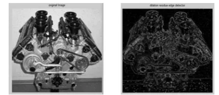
G. Dilation Residue edge detection
detected image using dilation residue method. The result is shown in figure 8.
[Fig.8 (a) Noisy Image (b) Output of Dilation Residue edge detector]
H. Erosion Residue edge detection
In case of erosion residue method, the image is dilated using the structuring element and the original image is subtracted from the eroded image which gives the edge detected image using erosion residue method. The result is shown in figure 9.
[Fig.9 (a) Noisy Image (b) Output of Erosion Residue edge detector]
I. Morphological Gradient operation (combination of
Dilation and Erosion)
In this method both dilation and erosion residue method are combined to gives good result. The final edge detected image is given in figure 10.
[Fig.10 (a) Noisy Image (b) Output of combination of all morphological operators]
We have applied the above methods not to the original image rather we have added the salt and pepper noise to make the result robust. We have applied all the methods to varieties of image including objects, scene images, animations etc.
[Fig.11 Edge detected output using all methods for ‘disnip.jpg’]
We have shown some of the sample image added with noise and their edge detection using different methods in figure 11, 12, 13 and 14.
[Fig.12 Edge detected output using all methods for ‘tiger.jpg’]
[Fig.13 Edge detected output using all methods for ‘house.jpg’]
[Fig.14 Edge detected output using all methods for ‘coins.jpg’]
The results shows that out of the conventional method canny edge detection methods showing a good response, but the morphological method giving better results where the combination of all morphological methods give much more clear edge detected images.
IV.CONCLUSIONS
REFERENCES
[1] Kangtai Wang, Wenzhan Dai, “Approach of image edge detection based on Sobel operators and grey relation”, Computer
Applications,26(5):1035-1036,2006.
[2] V. Torre and T. A. Poggio. “On edge detection”. IEEE Trans. Pattern Anal. Machine Intell., vol. PAMI-8, no. 2, pp. 187-163, Mar. 1986. [3] Mamta Juneja , Parvinder Singh Sandhu, “ Performance Evaluation of
Edge Detection Techniques for Images in Spatial Domain”,
International Journal of Computer Theory and Engineering, Vol. 1, December, 2009
[4] D. Marr and E.Hildreth. “Theory of Edge Detection”. Proceedings of the Royal Society of London. Series B, Biological Sciences,, Vol. 207, No. 1167. (29 February 1980), pp. 187-217.
[5] T. Peli and D. Malah. “A Study of Edge Detection Algorithm “ Computer Graphics and Image Processing, vol. 20, pp. 1-21, 1982. [6] A.Huertas and G. Medioni, “Detection of intensity changes with
sub-pixel accuracy using Laplacian-Gaussian masks” IEEE Transactions
on Pattern Analysis and Machine Intelligence. PAMI-8(5):651-664, 1986.
[7] John Canny, Member, IEEE, “A Computational Approach to Edge Detection”, IEEE Trans.on Pattern Analysis and Machine Intelligence, 8(1):679-697, 1986.
[8] S. Sridhar,”Digital Image Processing”,Oxford University Press, 2012
[9] R. C. Gonzalez and R. E. Woods. “Digital Image Processing”. 2nd ed.
Prentice Hall, 2002.
[10] ZHANG Yongliang,LIU Anxi, “Improved algorithm for computer digital lmage edge detection based on Prewitt operator”, Journal of PLA University of Science and Technology,6(1):45-47, 2005. [11] M. Heath, S. Sarkar, T. Sanocki, and K.W. Bowyer. “A Robust Visual
Method for Assessing the Relative Performance of Edge Detection Algorithms”. IEEE Trans. on Pattern Analysis and Machine
Intelligence, vol. 19, no. 12, pp. 1338-1359, Dec. 1997.
[12] E. Argyle. “Techniques for edge detection,” Proc. IEEE, vol. 59, pp. 285-286, 1971.
[13] F. Bergholm. “Edge focusing,” in Proc. 8th Int. Conf. Pattern
Recognition, Paris, France, pp. 597- 600, 1986.
[14] R. M. Haralick. “Digital step edges from zero crossing of the second directional derivatives,” IEEE Trans. on Pattern Anal. Machine Intell., vol. PAMI-6, no. 1, pp. 58-68, Jan. 1984.
[15] E. C. Hildreth, "Implementation of a theory of edge detection", M.I.T. Artificial Intell. Lab., Cambridge, MA, Rep. AI-TR-579,1980.. [16] M. Heath, S. Sarkar, T. Sanocki, and K.W. Bowyer. “Comparison of
Edge Detectors: A Methodology and Initial Study “. Computer Vision and Image Understanding, vol. 69, no. 1, pp. 38-54 Jan. 1998. [17] Kenneth R.Castleman. “Digital Image Processing”. Beijing : Tsinghua
university press, 1998.