Stomach Tumor Localization Method of a Support Vector Machine
Based on Capsule Endoscopy
Gong Chen*, Ye-Rong Zhang, and Bi-Yun Chen
Abstract—This study proposes a real-time method to solve the electromagnetic inverse scattering problem. This technique converts this problem into a regression problem using a support vector machine (SVM). The SVM-based solution successfully deals with the nonlinearity and ill-posedness inherent in this problem. Simulation results show the feasibility and effectiveness of the proposed method. The method can effectively locate the tumor target of the stomach regardless of the presence of noise. The positioning effect of the method improves as SNR increases. When the SNR is higher than 50 dB, noise minimally affects the results. Finally, the SVM prediction model is utilized to study the effect of the number of sampling locations on the prediction results. The results show that the more sampling locations, the better the prediction results.
1. INTRODUCTION
Electromagnetic inverse scattering [1–5] theory uses the scattered field detected by the scatterer to infer the spatial position of scatterers and their electromagnetic characteristics. This theory is widely adopted in seismology, medical imaging, target recognition, geophysical observation, and several nondestructive testing fields [6–8]. Electromagnetic inverse scattering has received much attention in the last 10 years, especially in the fields of target reconstruction and microwave imaging.
Gastrointestinal (GI) tract is a hollow and muscular conduit from the mouth to the anus. GI tract-related cancers, such as gastric, esophagus, and colon cancers, have been ranked as the third, fourth, and fifth major causes of male cancer deaths, respectively, whereas they have been ranked as the fourth, fifth, and sixth major causes of female cancer deaths, respectively, in Hong Kong in 2014 [9]. Tumors in the GI tract greatly threaten human health.
A novel endoscopy technique called wireless capsule endoscopy (WCE) was introduced in 2000 to diagnose GI tract cancers [10–14]. This technique consists of a short-focal-length camera, light source, and radio transmitter. When it is swallowed by a patient, the capsule relies on the peristalsis of the human GI tract as it moves through the esophagus, stomach, and finally drains out of the body. The camera takes photos of the GI tract and produces thousands of images in each examination. Spending two or more hours to review all the images would be time consuming for physicians. This scenario could also increase the chances of mistakes and misdiagnosis as physicians focus on a small part of the field for a long time. Hwang et al. [15] applied expectation maximization clustering on a dataset of approximately 15,000 capsule endoscopy images for blood detection to overcome the drawbacks of traditional endoscopy. Tjoa and Krishnan [16] proposed a polyp detection technique utilizing the Texture Spectrum and a Neural Network classifier. Igual et al. [17] described a method for analyzing the motion detected between the frames using principal component analysis to create high order motion data. The said researchers then employed relevance vector machine methods to classify the contraction
Received 26 June 2017, Accepted 6 September 2017, Scheduled 14 September 2017 * Corresponding author: Gong Chen ([email protected]).
sequences. Gono et al. proposed the narrow band image technology [18–20]. Li and Meng recently studied a computerized tumor detection system for WCE images, which exploits textural features and support vector machine (SVM)-based feature selection [21–24].
The aforementioned works have solved the detection of bleeding and ulcer in WCE images, but failed to obtain real-time imaging. Therefore, a new type of capsule endoscopy with ultra-wideband (UWB) [25–28] radar is utilized in this study for the first time. The medical imaging problem is a special case of electromagnetic inverse scattering problem. The inverse scattering problem is ill-posed because measurement data can only be collected in space, time, and frequency in a limited capacity. The regularization method must be used to solve the problem of non-unique solution caused by ill-posedness. The regularization parameters are all artificially set, and the values lack theoretical support, which causes difficulty in dealing with inverse scattering problems. This paper presents a method for locating stomach tumors based on SVM. This method [29, 30] is also utilized to establish statistical learning theory in the Vapnik-Chervonenkis dimension and structural risk minimization theories [31– 34]. SVM features a two-convex quadratic programming problem. Thus, SVM can obtain a global optimal solution and prevent the local optimal solution by neural networks. Furthermore, SVM has a regularization function that solves the regularization of the electromagnetic inverse scattering problem. This paper first describes the stomach tumor detection model. Then, imaging data can be obtained by utilizing the back projection (BP) algorithm [35, 36] and classified by SVM. Based on efficiency, BP algorithm requires 40 s to 60 s on the computer with Intel Core i5 CPU. After obtaining characteristic data, prediction process of SVM based on BP algorithm requires only 1 s. Therefore, the method not only can recognize the location and shape of the tumors, but also can meet requirements of real-time detection [37]. It can be employed for tumor positioning and help clinicians make decisions. The analysis shows that the problem is nonlinear and ill-conditioned. This study proposes a tumor detection method based on SVM. The effect of the number of sampling locations of the receiving antenna on the detection results is also investigated. Finally, the scenario which has noise pollution is also studied to simulate the actual scene.
2. FDTD MODE
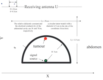
The method based on the data model should first have training and test data sets, which include input and output data pairs. The data pairs used for training and testing in this study are obtained by FDTD simulation [38, 39]. The simulation modeling of the stomach model is shown in Fig. 1. The relative permittivity of the tumor isε, and the conductivity isσ. The relative dielectric constant of the gastric isεb, and the conductivity isσb. The relative permittivity of the detection region isε0, and the
conductivity is σ0.
The scattering signal of the tumor is as follows:
Esca(xr, yr, xt, yt, ω) =k02
D
G(xr, yr, xt, yt, ω)×Etot(xr, yr, xt, yt, ω)×χ(x, y)dxdy, (1)
whereEscais the scattering field of the tumor,Etot the total scattering field in the imaging region,G(•) the green function for characterizing environment, (xt, yt) the location of the signal source, (xr, yr) the location of the receiving antenna, k0 the wave number, and the range of the detection area D is
[xmin, xmax]×[ymin, ymax],xr∈[−xm, xm], ω= 2πf,f the frequency of the transmitted signal. χ(•) is
the objective function that represents tumor information, and the expression is as follows:
χ(x, y) = εeq(x, y)−ε0
ε0 ,
(2)
where
εeq=ε(x, y)ε0−jσ
(x, y)
ω , (3)
Capsule with emission
source tumor
Abdominal
detection area on Stomach
Y
receiving
antenna
xm
-xm
ymin
xmax
xmin
ymin
Figure 1. Geometry model of gastric tumor imaging.
Esca at the sampling position also changes, which shows the mapping between B and Esca. In this
paper, FDTD is applied to simulate the stomach tumor scene, and B is changed continuously to obtain the correspondingEsca. The total signal is received by the receiving antenna at each sampling position, including the direct signal of the transmitting source, reflected signal of the gastric wall, and scattering signal of the tumor. Hence, the background subtraction method is employed to obtain Esca. Steps of background subtraction are as follows:
(i) The model with tumor is simulated by FDTD method, and all radar signals on receiving antenna are recorded.
(ii) Simulation is conducted again after removing the tumor from Step 1 model without changing the other parameters. All radar signals on receiving antenna are recorded again.
(iii) Scattering signal of tumor is obtained after subtraction of radar signal in Step 1 from radar signal in Step 2.
3. BASIC SVM PRINCIPLE
The basic idea of SVM is to transform the input variables into a high dimensional space via nonlinear transformations defined by the inner product functions. We seek a linear relationship between the input and output variables in this high-dimensional space [40–42].
Set the given training sample as{(xi, ti), i= 1,2, . . . , k}, wherexi∈RN is the input value, ti∈R
the corresponding target value, and k the sample number. First, a nonlinear mapping φ is utilized to map the data to a high-dimensional feature space. Linear regression is then performed in the high feature space. Let the regression function be the following:
f(x) =w, φ(x)+b, (4)
When SVMs are adopted to solve the regression problem, the loss function is introduced to detect the error between the fitting and target values. The loss functions mainly include Quadratic, Laplace, Huber, and are ε-insensitive [43–46].
The loss function used in this study isε-insensitive with a specific form presented as follows:
c(f(x)−y) =
0 if|f(x)−y| ≤ε
|f(x)−y| −ε otherwise . (5) Assume that all data are error free in accuracy, so the linear function is utilized to fit them. ε
represents accuracy, andy is the actual function value. The optimization regression function based on SVM is the principle satisfying the structural risk minimization according to statistical learning theory. The relaxation variables ξi and ξi∗ are introduced considering the allowable error. The minimization problem becomes the following:
min 1 2w
2+ C
k
i=1
(ξi+ξi∗)
s.t. f(xi)−ti≤ξi+ε, i= 1,2, . . . , k ti−f(xi)≤ξ∗i +ε, i= 1,2, . . . , k ξi, ξi∗ ≥0, i= 1,2, . . . , k
, (6)
where min indicates minimization;s.t.stands for constraints;Cis the penalty parameter. The Lagrange method is applied to solve the aforementioned constrained optimization problem, and the original problem is transformed into a dual problem as follows:
max − 1 2
k
i,j=1
(αi−α∗i)(αj −α∗j)φ(xi), φ(xj)+ k
i=1
(αi−α∗i)ti− k
i=1
(αi+α∗i)ε
s.t. k
i=1
(αi−α∗i) = 0 0≤αi, α∗i ≤C, i= 1,2, . . . , k
, (7)
whereαi and α∗i are Lagrange coefficients. Thus, the regression function f(x) is expressed as follows:
f(x) =
k
i=1
(αi−α∗i)φ(xi), φ(x)+b (8)
The inner product operations in the high-dimensional feature space should be calculated in the optimization of the upper type. At this point, a kernel function that satisfies the Mercer condition can be obtained to replace the inner product in the higher dimensional space as follows:
k(x, y) =φ(x), φ(y). (9)
This process avoids determining the exact mapping relationship of φ(x). The inner product operation in high dimensional space is solved ingeniously. The regression function is expressed as follows:
f(x) =
k
i=1
(αi−α∗i)K(xi, x) +b. (10)
For the new inputX, the output values are calculated by Equation (10).
When trained by SVM, the input is the scattered signal of the target. However, the target scattering signal obtained via FDTD modeling is a function of time, and thus several features should be extracted before training to represent the signal. This study uses amplitude E of the signal as the feature of the target scattering signal, so the features at all sampling locations are formed into vectors
4. EXPERIMENTS
4.1. Establishment of the Gastric Tumor Model
The stomach model is shown in Fig. 2. The length of the abdominal cavity is lx = 20 cm, whereas
its width isly = 12.5 cm. The relative dielectric constant and electrical conductivity of the abdominal
cavity are 36 and 7 S/m, respectively. A circular tumor model with a diameter of 1 cm in the coordinate site (0 and 4 cm) is obtained. The relative dielectric constant of the tumor is 50, and its electrical conductivity is 4 S/m [47]. The signal source is (0 cm, 0 cm) in a coordinate system. The receiver antenna is placed close to the outer side of the abdomen. A receiver antenna is arranged in the X
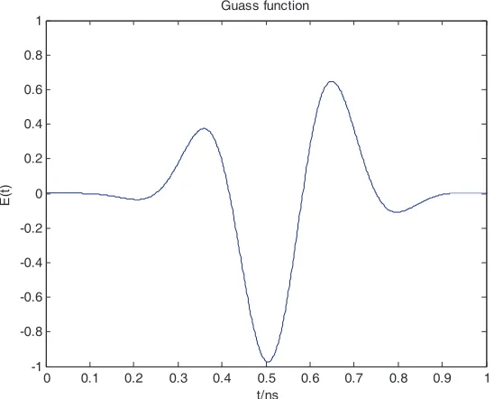
direction at 0.5 cm intervals. The aperture length is 22 cm, and the antenna number is U = 45. The transmitting signal is a sine-modulated Gauss pulse with a center frequency of 4 GHz and a width of 0.6 ns. The frequency and time domain waveforms of the signal are shown in Figs. 3 and 4, respectively. The space interval of the FDTD is dx =dy = 1 mm, and the time interval is dt = 19.25×10⁻¹². The calculation area is surrounded by a perfect matched layer absorbing boundary.
Y
s
X
Figure 2. Stomach model.
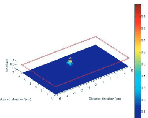
The imaging area is divided into a 400×300 mesh to improve the accuracy of target recognition. The feature vector is obtained according to the BP algorithm. The samples are then trained by the LibSVM toolbox. Tumor cells are considered positive, and healthy cells are considered negative, respectively. This condition means that 120,000 samples contain 377 positive samples and 119,623 negative samples. A total of 364 data samples, which must include the target information, are selected as the training set. The training model is utilized to predict the entire imaging area. The positive and negative classification accuracy values are 88.674% and 99.964%, respectively. The label of the positive class is 1, whereas that of the negative class is 0. The classification accuracy of the negative class is extremely high, which indicates that the ability to predict the medium is excellent. The classification accuracy of the positive class is slightly lower, but it can also meet the requirements of stomach imaging.
Figure 3. Frequency domain waveform of the transmitted signal.
0 0.1 0.2 0.3 0.4 0.5 0.6 0.7 0.8 0.9 1 -1
-0.8 -0.6 -0.4 -0.2 0 0.2 0.4 0.6 0.8 1
Guass function
t/ns
E(
t)
Figure 4. Time domain waveform of the transmitted signal.
The golden box indicates the location of the tumor.
Figure 5. Imaging results by the electric field intensity.
Figure 6. 3D imaging results by the electric field intensity.
4.2. Establishment of SVM Model
This study uses the SVM toolbox developed by Professor Lin Zhiren of Taiwan University to forecast classification accuracy. A total of 364 pixels are selected as training samples, including a certain number of positive samples. Appropriate classifier, kernel function, and normalization methods are selected according to results of several experiments.
Two categories of classifiers, namely, C-SVC and V-SVC, can be selected when SVM is considered as a classifier. BP algorithm is used to predict radar data using the two classifiers. After training, classification accuracies reach 88.674% and 85.321% for C-SVC and V-SVC, respectively. Accuracy rate of C-SVC is higher than that of V-SVC by 3.353%. Thus, C-SVC classifier is selected to train and predict data.
Figure 7. Imaging results by the prediction of the category labels.
four kinds of kernel function: linear kernel function, polynomial kernel function, radial basis kernel function (RBF), and sigmoid kernel function. SVM toolbox is used to train and predict the data obtained by BP algorithm with the four kinds of kernel functions. Classification accuracies of the four kernel functions total 67.745%, 64.823%, 88.674%, and 50.015%, respectively. Thus, RBF is selected for the SVM model.
Penalty parameter C and the parameter γ in RBF can be obtained by optimization of genetic algorithms or networks. As stomach tumor imaging requires real-time imaging, longer delay results in poorer disease prognosis. Therefore, this paper adopts a network optimization method with shorter computation time.
According to machine type classifications, kernel functions, normalization, and parameter selection tests, high classification accuracy in obtaining parameters of C and γ can be achieved with the use of C-SVC classification, RBF, and network optimization method. Radar data obtained by BP algorithm are trained to obtain the SVM model, namely, modelBP.
4.3. Location of Tumor Model
This study only focuses on the tumor localization problem. The coordinates of the target center of the tumor are set at (x, y). The tumor position in the training samples varies as follows:
xp=−5 +pΔx, p= 1,2, . . .
yp=sqrt(52−pΔx2), p= 1,2, . . . (11)
Similarly, the tumor location in the test sample changes as follows:
xq =−4.5 +qΔy, q = 1,2, . . .
yq =sqrt(4.52−qΔy2), q= 1,2, . . . (12)
where Δx = 0.1 cm, Δy = 0.09 cm, and p = q = 100. The Gauss kernel function is used in the SVM training, which is one of the Radial Basis Functions (RBF), and the expression is presented as follows:
K(xi, xj) = exp(−γxi−xj2), (13) where γ is a width parameter and controls the radial range of the function. xi is the predictive value, and xj is the central value of the kernel function.
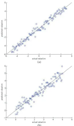
(a)
(b)
Figure 8. Actual and predictive values of the tumor center compared to the graph: (a) abscissa, (b) ordinate.
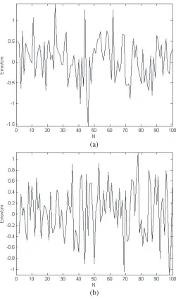
The black line in the figure represents the actual value, whereas the circle represents the predicted value. The said figure shows that the predicted value has only a small deviation from the actual value. Hence, the use of SVM for predicting tumor location is feasible and effective. Once the training process is completed, predicting tumor location only takes a few seconds, so the algorithm can be employed for real-time detection. We then list the prediction errors of the 100 test data items. The target location of the stomach tumor can be correctly located by SVM, as shown in Fig. 9, and the prediction error is within 0.2 cm.
(a)
(b)
Figure 9. Prediction error: (a) abscissa, (b) ordinate.
the receiving antenna is extremely far would it receive an extremely weak scattering signal from the tumor. The interaction between the tumor and abdominal cavity is predominant at this time. This will cause strong interference to the received signal and affects prediction accuracy.
For a further quantitative analysis of prediction errors, we define relative prediction errors as follows:
ηx = |xact−xpre|
lx
ηy = |yact−ypre|
ly
, (14)
where (xact, yact) is the actual location of the tumor center, (xpre, ypre) the predictive location for the tumor center, and lx and ly are the width and length of the model, respectively. The maximum, minimum, and average relative errors of the tumor target prediction are listed in Table 1. This table shows that the stomach tumor imaging algorithm based on SVM has high fidelity.
(a)
(b)
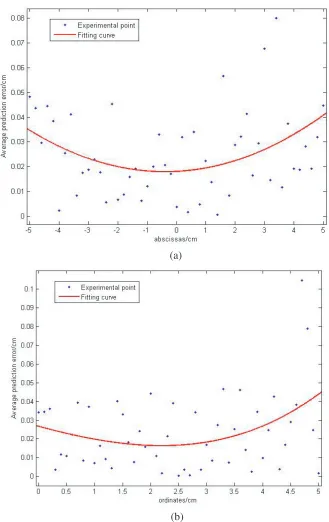
Figure 10. Average prediction error: (a) abscissa, (b) ordinate.
Table 1. Relative error analysis of predicting the location of the tumor center.
Max Min Average
ηx 0.1543 0.0069 0.0523
Table 2. Relative error analysis of predicting the location of the tumor center in case of noise.
SNR/dB 5 10 20 30 65 80
ηx 0.614 0.589 0.477 0.269 0.029 0.031 ηy 0.399 0.385 0.323 0.240 0.039 0.038
error of the localization of the stomach tumor using this imaging algorithm is also presented in Table 2. This table shows that the proposed method can effectively locate stomach tumors even at low SNR. With the increase of SNR, its positioning effect will be better. When SNR is higher than 50 dB, noise minimally affects the results. Thus, the proposed method is robust.
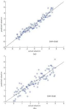
We add the SNR noise level of 30 dB in the scattering signal. The training model is utilized to predict the 100 data items in the test sample. The results are shown in Fig. 11, where the projections
(a)
(b)
are the abscissa and ordinate of the target center.
The aforementioned scenario studies the number of sampling positions of the receiving antenna (U = 45). What will happen to the result when theU changes? We investigate the effect of the number of sampling locations of U on tumor localization in the following. The conditions of U = 5, 10, 15, 20, 25, 30, 35, 40, 45 are studied. The relative root mean square error (RMSE) of the abscissa and ordinate
(a)
(b)
of the tumor center is defined as follows:
eRMS,x=
1
M M
i=1
xiact−xipre lx
2
eRMS,x=
1
M M
i=1
yiact−yipre ly
2
, (15)
where (xiact, yiact) is the actual location of the tumor target, (xipre, yipre) the predictive location of the tumor target, M the number of the test samples, and lx and ly are the model length and width, respectively. The relationship between the RMSE and sample location number U is shown in Fig. 12.
With the increase in number of sampling locations, the prediction error decreases, and the prediction
(a)
(b)
performance improves. Results show that the detection accuracy of a gastric tumor can be improved by increasing the number of receiving antennas.
The relative RMSE values of the predicted results under different SNR values are compared below. The proposed method can localize stomach tumors even at low SNR, as shown in Fig. 13. As SNR increases, RMSE decreases, and positioning effect improves (i.e., this method is robust).
We have also studied the prediction error with respect to the training size. The experimental results are shown in Fig. 14. It can be seen that with the increase in the size of the training set, ERMS decreases.
(a)
(b)
5. CONCLUSION
Considering the nonlinearity and ill-posedness of electromagnetic inverse scattering problems, this paper presents a method for detecting stomach tumors based on SVM. This method reconstructs the nonlinear problem into a convex quadratic programming problem. Thus, the global optimal solution is obtained, and the nonlinear local solution is successfully solved. In SVM, overfitting occurs sometimes when the object function is used. At this point, SVM parameters are often limited, making the SVM model simpler. This is called regularization. The algorithm contains the regularization idea, which provides an advantageous approach to solve the ill-posed problem in inverse scattering problems. Simulation results show that the proposed method can detect the tumor targets in the stomach regardless of the presence of noise, which proves the feasibility and robustness of the algorithm. The effect of the number of sampling locations of the receiving antenna on the detection of gastric tumor is also studied. The numerical results indicate that better positioning effect is achieved with increased number of sampling locations.
REFERENCES
1. Caorsi, S., M. Donelli, A. Lommi, and A. Massa, “Location and imaging of two-dimensional scatterers by using a particle swarm algorithm,” Journal of Electromagnetic Waves and Applications, Vol. 18, No. 4, 481–494, 2004.
2. Craddock, I. J., M. Donelli, D. Gibbins, and M. Sarafianou, “A three-dimensional time domain microwave imaging method for breast cancer detection based on an evolutionary algorithm,”
Progress In Electromagnetics Research M, Vol. 18, 179–195, 2012.
3. Rocca, P., M. Donelli, G. L. Gragnani, and A. Massa, “Iterative multi-resolution retrieval of non-measurable equivalent currents for the imaging of dielectric objects,” Inverse Problems, Vol. 25, No. 5, 2009.
4. Franceschini, G., M. Donelli, R. Azaro, and A. Massa, “Inversion of phaseless total field data using a two-step strategy based on the iterative multiscaling approach,”IEEE Transactions on Geoscience and Remote Sensing, Vol. 44, No. 12, 3527–3539, Dec. 2006.
5. Franceschini, G., M. Donelli, R. Azaro, and A. Massa, “Inversion of phaseless total field data using a two-step strategy based on the iterative multiscaling approach,”IEEE Transactions on Geoscience and Remote Sensing, Vol. 44, No. 12, 3527–3539, 2006.
6. Bolomey, J. C., “Recent european developments in active microwave imaging for industrial, scientific, and medical applications,” IEEE T. Microw. Theory, No. 37, 2109–2117, Dec. 1989. 7. Ram, S. S., Y. Li, A. Lin, and H. Ling, “Doppler-based detection and stacking of humans in
indoor environments,” Journal of the Franklin Institute — Engineering and Applied Mathematics, Vol. 345, No. 6, 679–699, 2008.
8. Le, C., T. Dogaru, L. Nguyen, and M. A. Ressler, “Ultrawideband (UWB) radar imaging of building interior: Measurements and predictions,” IEEE Transactions on Geoscience and Remote Sensing, Vol. 47, No. 5, 1409–1420, 2009.
9. National Breast Cancer Coalition (NBCC), URL: http://www.stopbreast- cancer.org, 2014. 10. Iddan, G., G. Meron, and A. Glukhovsky, “Wireless capsule endoscopy,”Nature, Vol. 405, 417–417,
May 2000.
11. Yujiri, L., “Passive millimeter wave imaging,”IEEE MTT-S International Microwave Symposium, Vol. 4, 98–101, Jun. 2006.
12. Hu, C., L. Liu, and B. Sun, “Compact representation and panoramic representation for capsule endoscope images,” Int. J. Inf. Acquisit., Vol. 6, 257–268, 2009.
14. Atasoy, S., B. Glocker, S. Giannarou, D. Mateus, A. Meining, G. Yang, and N. Navab, “Probabilistic region matching in narrow-band endoscopy for targeted optical biopsy,” Proc. MICCAI, 499–506, 2009.
15. Hwang, S., J. Oh, J. Cox, S. J. Tang, and H. F. Tibbals, “Blood detection in wireless capsule endoscopy using expectation maximization clustering,” Proc. SPIE, Vol. 6144, 2006.
16. Tjoa, P. M. and M. S. Krishnan, “Feature extraction for the analysis of colon status from the endoscopic images,”Biomed. Eng. Online, Vol. 2, 2003.
17. Igual, L., S. Segul, J. Vitria, F. Azpiroz, and P. Radeva, “Eigenmotion-based detection of intestinal contractions,” Proc. CAIP, Springer LNCS, Vol. 4673, 293–300, 2007.
18. Gono, K., “Multifunctional endoscopic imaging system for support of early cancer diagnosis,”IEEE J. Sel. Topics Quant. Electron, Vol. 14, No. 1, 62–69, Jan. 2008.
19. Gono, K., T. Obi, M. Yamaguchi, N. Ohyama, H. Machida, Y. Sano, S. Yoshida, Y. Hamamoto, and T. Endo, “Appearance of endhanced tissue features in narrow band endoscopic imaging,” J. Biomed. Opt., Vol. 9, 568–577, May 2004.
20. Gono, K., K. Yamazaki, N. Doguchi, T. Nonami, T. Obi, M. Yamagichi, N. Ohyama, H. Machida, Y. Saono, S. Yoshida, Y. Hamamoto, and T. Endo, “Endoscopic observation of tissue by narrow band illumination,”Opt. Rev., Vol. 10, 211–215, 2003.
21. Li, B. and M. Q.-H. Meng, “Tumor recognition in wireless capsule endoscopy images using textural features and SVM-based feature selection,” IEEE Trans. on Information Technology in Biomedicine, Vol. 16, No. 3, 323–329, May 2012.
22. Li, B. and M. Q.-H. Meng, “Computer aided detection of bleeding regions in capsule endoscopy images,”IEEE Trans. Biomed. Eng., Vol. 56, No. 4, 1032–1039, Apr. 2009.
23. Li, B. and M. Q.-H. Meng, “Texture analysis for ulcer detection in capsule endoscopy images,”
Image Vis. Comput., Vol. 27, No. 9, 1336–1342, Aug. 2009.
24. Li, B. and M. Q.-H. Meng, “Computer-based detection of bleeding and ulcer in wireless capsule endoscopy images by chromaticity moments,” Comput. Bilo. Med., Vol. 39, No. 2, 141–147, Feb. 2009.
25. Kanaan, M. and M. Suveren, “In-body ranging for ultra-wide band wireless capsule endoscopy using a neural network architecture,” 10th International Symposium on Medical Information and Communication Technology (ISMICT), 1–5, Worcester, USA, Mar. 20–23, 2016.
26. Kanaan, M. and M. Suveren, “Ranging for in-body localization of ultra wide band wireless endoscopy capsules using neural networks,”24th Signal Processing and Communication Application Conference, (SIU-2016), Zonguldak, Turkey, May 16–19, 2016.
27. Kanaan, M. and M. Suveren, “In-body ranging with ultra-wideband signals: Techniques and modeling of the ranging error,”Wireless Communications and Mobile Computing, Vol. 2017, 1–15, 2017.
28. Kanaan, M. and M. Suveren, “A novel frequency-dependent path loss model for ultra wideband implant body area networks,” Measurement, Vol. 68, 117–127, 2015.
29. Massa, A., A. Boni, and M. Donelli, “A classification approach based on SVM for electromagnetic sub-surface sensing,”IEEE Transactions on Geoscience and Remote Sensing, Vol. 43, No. 9, 2084– 2093, Sep. 2005.
30. Donelli, M., F. Viani, P. Rocca, and A. Massa, “An innovative multi-resolution approach for DoA estimation based on a support vector classification,”IEEE Trans. Antennas Propag., Vol. 57, No. 8, 2279–2292, Aug. 2009.
31. Wang, L.,Support Vector Machines: Theory and Applications, Springer-Verlag, New York, 2005. 32. Jain, A. K. and D. Zongker, “Feature selection, evaluation, application, and small sample
performance,”IEEE Trans. PAMI, Vol. 19, No. 2, 153–158, Feb. 1997.
33. Dash, M. and H. Liu, “Feature selection for classification,” Intell. Data Anal., Vol. 1, 131–156, 1997.
35. Lei, W., C. Huang, and Y. Su, “A real-time BP imaging algorithm in SPR application,” IEEE International Geoscience and Remote Sensing Symposium, 1734–1737, 2005.
36. Ahmad, F., M. Amin, and S. Kassam, “A beamforming approach to stepped-frequency synthetic aperture through-the-wall radar imaging,” IEEE International Workshop on Computational Advances in Multi-sensor Adaptive Processing, 24–27, 2005.
37. Salucci, M., N. Anselmi, G. Oliveri, P. Calmon, R. Miorelli, C. Reboud, and A. Massa, “Real-time NDT-NDE through an innovative adaptive partial least squares SVR inversion approach,” IEEE Transactions on Geoscience and Remote Sensing, Vol. 54, No. 11, 6818–6832, Nov. 2016.
38. Sullivan, D. M., “Electromagnetic simulation using the FDTD method,”IEEE Mircowave Theory and Techniques Society, 2000.
39. Chamma, W. A., “FDTD modeling of a realistic room for through-the-wall radar applications,”
International Journal of Numerical Modelling: Electronic Networks Devices and Fields, Vol. 22, No. 2, 159–174, 2009.
40. Vapnik, V. N.,Estimation of Dependencies Based on Empirical Data, Springer-Verlag, Berlin, 1982. 41. Vapnik, V. N.,The Nature of Statistical Learning Theory, Springer-Verlag, 1995.
42. Vapnik, V. N., S. E. Golowich, and A. Smith, “Support vector method for function approximation, regression estimation and signal processing,”Advances in Neural Information Processing Systems, Vol. 9, 281–287, 1997.
43. Cristianini, N. and J. S. Taylor, An Introduction to Support Vector Machines and Other Kernel-based Learning Methods, Cambridge University Press, New York, 2000.
44. Smola, A. J., B. Scholkopf, and K. R. Muller, “The connection between regularization operators and support vector kernels,” Neural Networks, Vol. 11, No. 4, 637–649, 1998.
45. Bermani, E., A. Boni, A. Kerhet, and A. Massa, “Kernels evaluation of SVM-based estimators for inverse scattering problems,” Progress In Electromagnetics Research, Vol. 49, 372–375, 2007. 46. Suykens, J. A. and J. Vandewalle, “Recurrent least squares support vector machines,” IEEE
Transactions on Circuits Systems, Vol. 47, No. 7, 1109–1114, 2000.