BACTERIAL FORAGING OPTIMIZATION ALGORITHM FOR NEURAL NETWORK LEARNING ENHANCEMENT

(1)

International Journal

of

Innovative Computing

Journal Homepage: http://se.cs.utm.my/ijic

8

BACTERIAL FORAGING OPTIMIZATION ALGORITHM FOR

NEURAL NETWORK LEARNING ENHANCEMENT

Ismail Ahmed Al-Qasem Al-Hadi

Faculty of Computer Science and Information Technology University Putra Malaysia

Selangor, Malaysia [email protected]

Siti Zaiton Mohamed Hashim

Soft Computing Research Group, Faculty of Computer Science and Information Systems, UTM

Johor, Malaysia [email protected]

Abstract— Backpropagation algorithm is used to solve many

real world problems using the concept of Multilayer Perceptron. However, the main disadvantages of Backpropagation are its convergence rate is relatively slow, and it is often trapped at the local minima. To solve this problem, in literatures, evolutionary algorithms such as the Particle Swarm Optimization algorithm has been applied in feedforward neural network to optimize the learning process in terms of convergence rate and classification accuracy but this process needs longer training time. To provide alternative solutions, in this study, Bacterial Foraging Optimization Algorithm has been selected and applied in feedforward neural network to enhance the learning process in terms of convergence rate and classification accuracy. One of the main processes in Bacterial Foraging Optimization algorithm is the chemotactic movement of a virtual bacterium that makes a trial solution of the optimization problem. This process of chemotactic movement is guided to make the learning process of Artificial Neural Network faster. The developed Bacterial Foraging Optimization Algorithm Feedforward Neural Network is compared against Particle Swarm Optimization Feedforward Neural Network. The results show that Bacterial Foraging Optimization Algorithm gave a better performance in terms of convergence rate and classification accuracy compared to Particle Swarm Optimization Feedforward Neural Network.

Keywords— Bacterial foraging; particle swarm; neural network; backpropagation.

I.INTRODUCTION

Artificial Neural Network (ANN) is a model of information processing simulated by the biological nervous system. Feedforward Neural Network (FFNN) has been commonly used in several fields such as control applications [1], dynamic problems [2] and power systems [3]. This is because ANN has the ability to closely approximate unknown function to each degree of desired accuracy [4]. There are many calculations, which are very complex, nonlinear and parallel that could be

(2)

9 from predators [11]. Bacterial Foraging Optimization

Algorithm (BFOA) has been widely used for global optimization [12].

II.BFOA USING FEED-FORWARD NEURAL NETWORK

This section describes the background of the research problem. The issues of neural network and related techniques used in solving the problem of error convergence are discussed. This section also discusses the concepts of artificial neural network and algorithms used to enhance neural network learning. The optimization algorithms like PSO, GA, BP, and BFOA are explained particularly on how they are used to improve the learning [13].

a) Artificial Neural Network

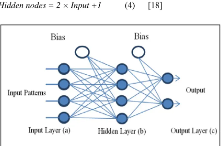
An artificial neuron represents a biological neuron model. Any neuron obtains signals from the surroundings or the nearest neurons. The neuron collects all received signals, and computes a net input signal as a function of the individual weights. The net input signal provides input to the activation function which calculates the output signal of this neuron. Fig. 1 represents the architecture of ANN. ANN is a computerized form of the nervous system. ANN describes a continuous function approximated with a small error, and through the process of training ANN is updating all the values of its nodes in order to try to obtain possible values to reduce the error. This error comes as a result of the difference between the output value of ANN and the target attribute [14]. Neural network consists of many neurons (nodes) that are parallel set of simple processing units, which are structured and joined in a network topology [15]. Usually, ANN contains three layers that are input, hidden, and output layers respectively. The input layer consists of many nodes that are determined by data set. Each node has linked weights to all nodes in the next layer and also one bias linked to the same nodes of the next layer. Bias nodes always have an output of one node and they are connected to all nodes to their respective layer. The weights on the connections from bias nodes are called bias weights [16]. Fig. 1 shows the simple architecture of ANN.

All weights that are linked to each node are computed to give the summation of this node (x), and then the activation function of this node is computed. The same operation for other nodes, the value of x equation is computed first then the activation function of the same node is computed by obtaining the activation function of the output node [17]. There are many types of the activation functions such as a step function, a sign function and a sigmoid function. The common activation function is a sigmoid function as shown in Eq. 1:

x

e

x

f

₋

+

=

1

1 )

(

(1)

Where x is an input which gets by Eq. 2 as follows :

∑

=

+

=

n

b

b b ab

O

w

x

1

θ

The error is calculated using Eq. 3 to measure the differences between target output and actual output, which is produced in Feedforward part as follows :

∑

−

= ₍_Target_output _Actual_output₎2 2

1

Error

(3)

Normally, the numbers of nodes in the input layer and the output layer are fixed depending on the number of inputs and the number of outputs of its dataset, respectively. For the number of nodes in hidden layer that Kolmogorov theorem is used in this research which shown in Eq. 4 as follows:

Hidden nodes = 2 × Input +1 (4) [18]

Fig. 1. simple architecture of ANN

b) Bacterial Foraging Optimization Algorithm

In 2002, Passino proposed a new algorithm for distributed optimization and control; that is, BFOA. The BFOA is a recent evolutionary computing method which depends on the foraging behavior of Escherichia coli (E. coli) bacteria in human intestine. Natural selection tends to reduce animals with poor foraging strategies and support the propagation of genes of those animals that have rich foraging strategies, while they are more expected to have reproductive success. After many generations, poor foraging strategies are either eliminated or formed into skillful ones. This activity of foraging led the researchers to use it as optimization process. The E. coli bacteria that live in our intestines also undergo a foraging strategy. The control system on the E. coli that dictates how foraging should proceed [13].

1. Chemotaxis : A bacterium normally attracts to move to the nearest sources of nutrients. The process is the main operation that represents the movement of a bacterium achieved through alternate swimming and tumbling by flagella. The bacterium moves toward the optimum error (source of nutrient). It contains two steps as follows:

(3)

10 of the bacterium to the next location, Eq. 5 represents this

step as follows:

) ( ) ( (i) C(i) l) k, (j, l) k, 1, (j

×

i i T i i Δ Δ Δ + = + θ

θ ₍₅₎

Where

Δ (i), Δ : Random vectors on [-1, 1]

) ( ) ( (i) i i T _Δ Δ Δ

: The unit walk in the random direction C: Run length unit

l) , k , (j i

θ _{: It may represent by P (i, j, k, ell)}

) l , k , 1 j ( + i

θ _{: It may represent by P (i, j+1, k, ell)} that represents the next location of bacterial.

• Swimming: A bacterium continues to move in a particular direction if the error is minimized (rich in nutrients). Exactly, if the next location is richer than the first location then other swimming steps in the same direction is taken, and it can repeat this process until it completes the chemotactic steps. However, if the next location is poorer than the first location then the bacteria change this direction for avoiding the poor location that means tumble.

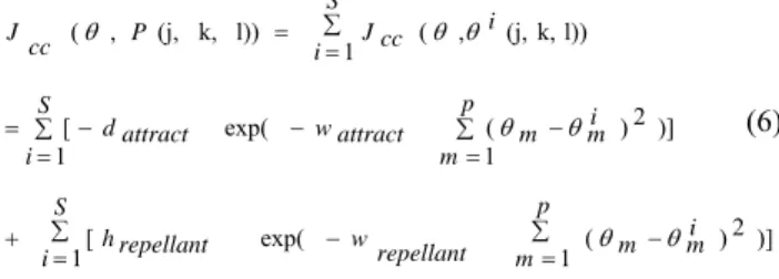
2. Swarming: When a group of E. coli bacteria is located in the semisolid agar having a sensor to a dangerous place, they shift from the center to outwards direction in a moving ring of bacteria by following the nutrient gradient produced by the group of bacteria which consume the nutrient. Furthermore, the bacteria drop attractant aspartate if high levels of succinate are used as the nutrient, which leads the bacteria to concentrate into groups and hence move as concentric patterns of groups with high bacterial density. The spatial order depends on both the outward movements of the ring and the local releases of the attractant, which functions as an attraction signal between bacteria to gather into a swarm. [19]. The Eq. 6 is the cell to cell attraction function that represents a signal to the rich location or poor location.

)] 1 2 ) ( exp( 1[ )] 1 2 ) ( exp( 1 [

1 ( , (j,k,l)) l)) k, (j, , ( ∑ = − − ∑ = + ∑ = − − ∑ = − = ∑ = = p m i m m repellant w S

i hrepellant

p m i m m attract w S i attract d S i i cc J P cc J θ θ θ θ θ θ θ Where

d attract depth attractant to set a magnitude of secretion of

attractant by a cell

w attract width attractant to set how the chemical cohesion

signal diffuses (smaller makes it diffuse more)

h repellant height repellant to Set repellant (a tendency to

avoid nearby cell)

w repellant width repellant to Make the small area where the

cell is relative to diffusion of chemical signal S number of bacterial

p dimension of the search space or ANN

m members of bacterium number i

i

m members of all bacterial

• Reproduction : The fitness values of the bacteria are sorted in array order arrange from small to big value. The lower half of the bacteria have higher fitness which dies and the remaining bacteria, which are the half population, allowed to split into two equal parts with the same values. This makes the population of bacteria constant. The health is computed by using Eq. 7 as follows:

(

)

∑+ = = 1 1 , , , c N j l k j i J i health

J (7)

Where N C is the chemotactic steps and j is the value of error.

• Elimination and Dispersal: A few bacteria in the real world have probability and dispersed to new locations. The elimination process starts with generating the random vector of size 1×S. Then the elements of the vector are sorted in the climbing order. After that, the index is located to match the bacteria that are sorted based on the healthy. Then, choose the positions of the bacterium matching to the obtained index. They are swapped on the optimization domain with the randomly generated positions include [-1, 1]. These positions are treated as the current best positions. Finally, by completing the loops, the best value in each iteration can be tracked and the best value among them can be declared as the optimal solution.

III.Data Preparation

The problem is represented by the dataset because universal data has been applied for classification, clustering and other. Each dataset contains a number of attributes that represent the input patterns that equal to the input nodes of ANN. Furthermore, every dataset contains a different number of instances or patterns based on the kind of dataset. In this research, five classification datasets are chosen in order to classify the weights in ANN by using two algorithms. The datasets used in this research are XOR, Balloon, Cancer, Heart and Ionosphere. These datasets are taken from the center of Machine Learning and Intelligent Systems "http://archive.ics.uci.edu/ml/datasets.html". Each dataset is applied with BFOANN and PSONN implementations.

IV.Methodology of BFOANN

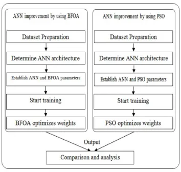
Fig. 2 is the framework of this study which implemented to integrate BFOA in ANN. This work used five datasets XOR, Balloon, Cancer, Heart and Ionosphere validate the proposed method.

(4)

11 Fig. 2.A Framework of the study

A. Initialization of the BFOANN

The algorithm of BFOANN depends on a multidimensional array. Therefore, this model of BFOA based ANN uses five dimensions. First dimension based on a dimension of neural network that calculates by use the Eq. 8:

Dimension = (Input × Hidden)+(Hidden × Output)+Hidden+ Output (8)

The second dimension of a multidimensional array is set to the number of bacteria, and this number should be an even number in order to be divided by 2. The third dimension is set to the number of chemotactic steps. The fourth dimension is set to the number of reproduction steps. The fifth dimension is set to the number of elimination and dispersal events. For initializing a population of bacteria, members of all bacteria are initialized by a random number between 0 to 1 for each member, and this initialization only for first and second dimensions, and the remain dimensions will be created automatically using BFOANN model.

Table 1: ANN ARCHITECTURE

Type of dataset

Dataset patterns _Input

nodes

Hidden nodes

Output nodes

Training Testing

XOR 6 2 3 7 1

Balloon 12 4 4 9 1

Cancer 120 30 9 19 1

Heart 100 25 13 27 1

Ionosphere 100 25 34 69 1

Table 1 shows the ANN architecture for both PSONN and BFOANN that are used five layers and same architectures for XOR, Balloon, Cancer, Heart and Ionosphere datasets.

B. BFOANN Learning Process: The process of ANN is represented by obtaining one bacterium. The members of this bacterium equal to the weights and bias of ANN (dimension). The training process is represented by a set of train patterns from dataset with these weights (bacterium) to give the error of this bacterium. The whole errors of bacterial are compared to knowing which bacterium gives the optimum weight. It is the best bacterium, and this bacterium is the best weights for this iteration. For the iteration that stops with limited error, the best bacterium gives the optimum error which equal or less than the limited error. However, final iteration, the best bacterium gives the optimum error that is less than the limited error. The test set is used for testing the best bacterium after completing the train BFOANN to evaluate the performance of optimum weights that introduced by train ANN. Fig. 3 shows the example of the process for BFOA based on ANN and how to optimize the weights. Table 2 and Table 3 show the initial parameters of PSONN and BFOANN which are used in this work to show the effect of BFOANN for optimizing the neural network.

Table 2: Initialize PSONN Parameters

Parameters of

PSONN XOR Baloon Cancer Heart

Ionosphe re

N. of Particles 20 20 20 20 20 Dimension 21 55 210 406 2485

Delta 0.1 0.1 0.1 0.1 0.1 C1(acceleration

constant) 2 2 2 2 2

C2 (acceleration

constant) 2 2 2 2 2

Minimum Error 0.005 0.005 0.005 0.005 0.005 Maximum

Iteration 1000 500 500 1000 1000

(5)

12 Table 3: Initialize BFOANN Parameters

Parameters of

BFOANN XOR Balloon Cancer Heart Ionosphere

Number of

bacterial (S) 20 20 20 4 4

Dimension (p) 21 55 210 406 2485

Chemotactic

steps (Nc) 8 4 4 4 4

The length of

a swim (Ns) 4 4 4 4 4

Reproduction

steps (Nre) 2 2 2 2 2

Elimination-dispersal (Ned) 2 2 2 2 2

Probability (Ped) 0.25 0.25 0.25 0.25 0.25

Run length

unit (C) 0.08 0.40 0.5 0.3 0.3

Minimum Error 0.005 0.005 0.005 0.005 0.005

Maximum Iteration 1000 500 500 200 200

V. EXPERIMENTALRESULT

This study describes the experiment conducted and results obtained in the validation process of the proposed BFOANN. The result is compared against results of PSONN. BFOA is implemented to optimize the learning of neural network. XOR, Balloon, Cancer, Heart and Ionosphere datasets are utilized as training and testing data for proving the proposed BFOANN model. The performance of the BFOANN and PSONN are compared and analyzed regarding to terms of convergence rate and classification accuracy. The experimental results for BFOANN and PSONN are explained in 5 sections as follows:

1 Results on XOR Dataset

The results of this study show the efficiency of BFOA and PSONN on the same data. From Table 4, BFOANN converges at iteration of 15 while PSONN converges at iteration of 41 for the overall process of learning. Both algorithms are converged by using the minimum error criteria. For the classification percentage, it illustrates that BFOANN is better than PSONN with 97.03 % compared to 95.17 %. Fig. 4 shows the process of learning for each algorithm. In BFOANN, all bacteria work together to get the optimum error (rich food) by helping a signal from cell to cell attraction function. In PSONN, all particles work together to find the optimum error (gbest). However, BFOANN is better than PSONN in convergence rate.

Table 4: Results of BFOANN and PSONN on XOR dataset

Learning Iteration

BFOANN PSONN

Train Test Train Test

15 1 41 1 Error Convergence 0.004320 0.5000 0.004898 0.2619

Classification (%) 97.03 49.96 95.17 57.06

Fig. 4. Convergence of XOR dataset

2 Results on Balloon Dataset

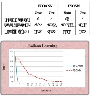
Table 5 shows that BFOANN converges at iteration of 3 while PSONN converges at iteration of 35 for the overall process of learning. Both algorithms are converged by using the minimum error criteria. For the classification percentage, it illustrates that BFOANN is better than PSONN with 99.21% compared to 97.69%. Fig. 5 shows the process of learning for each algorithm. In BFOANN, 20 bacteria work together to get the optimum error (rich food) by 3 iterations only, any iteration all bacteria swarm toward the minimum error during four loops where bacteria depend on the array of five dimensions. In PSONN, 20 particles at 35 iterations work together to find the optimum error (gbest); but BFOANN is better than PSONN in convergence rate.

Table 5: Results of BFOANN and PSONN on Balloon dataset

Learning Iteration

BFOANN PSONN

Classification (%) 99.21 29.22 97.69 9.32

Fig. 5. Convergence of Balloon dataset [13]

3. Results on Cancer Dataset

(6)

13 illustrates that BFOANN is better than PSONN with 99.71%

compared to 99.68%. Fig. 6 shows the process of learning for each algorithm. In BFOANN, 20 bacteria swarm toward the optimum error (rich food) by helping a signal from cell to cell attraction function. In PSONN, 20 particles work together at any iteration to find the optimum error (gbest). However, BFOANN is better than PSONN in convergence rate.

Table 6: Results of BFOANN and PSONN on Cancer dataset

Learning Iteration

BFOANN PSONN

Train Test Train Test

Classification (%) 99.71 95.90 99.68 63.71

Fig. 6. Convergence of Cancer dataset

4. Results on Heart Dataset

Table 7 shows that BFOANN converges at iteration of 500 while PSONN converges at iteration of 1000 for the overall process of learning. Both algorithms are converged by using the minimum error criteria. For the classification percentage, it illustrates that BFOANN is better than PSONN with 94.10% compared to 91.18%. Fig. 7 shows the process of learning for each algorithm. In PSONN, 20 particles work together at any iteration to find the optimum error (gbest) but BFOANN is better than PSONN in convergence rate because BFOANN takes half the number of PSONN iterations to reach to the optimum error.

Table 7: Results of BFOANN and PSONN on Heart dataset

Learning Iteration

BFOANN PSONN

500 1 1000 1

Error Convergence 0.88612 1.4909 1.98876 4.9257

Classification (%) 94.10 83.26 91.18 59.31

Fig.7. Convergence of Heart dataset

4. Results on Ionosphere Dataset

From Table 8 shows that BFOANN converges at iteration of 152 while PSONN converges at iteration of 1000 for the overall process of learning. Both algorithms are converged by using the minimum error criteria. For the classification percentage, it illustrates that BFOANN is better than PSONN with 99.40% compared to 94.41%. Fig. 8 shows the process of learning for each algorithm. In PSONN, 20 particles work together at any iteration to find the optimum error (gbest) but BFOANN is better than PSONN in convergence rate because BFOANN takes a small number of iterations compared to PSONN iterations to reach to the optimum error.

Table 8: Results of BFOANN and PSONN on Ionosphere dataset

Learning Iteration

BFOANN PSONN

Classification (%) 99.40 91.48 94.41 48.09

Fig. 8. Convergence of Ionosphere dataset

VI.DISCUSSION

(7)

14 same dataset. BFOANN parameters also are selected

depending on the dataset and the problem to be enhanced. These parameters can be changed consequently to succeed the better optimization. However, to get best evaluation, both algorithms use the same parameters for all five datasets. For BFOANN, the convergence rate is achieved by the suited number of iterations compared to PSONN which use more iterations. This is to ensure that the convergence rate of BFOANN and its error convergence is better with high classification percentage compared to PSONN overall process.

VII.CONCLUSION

In this paper, BFOANN is implemented on five types of datasets by using the architecture of Kolmogorov theorem. From the current results , BFOANN has good performance in ANN learning in terms of convergence rate and correct classification percentage. Furthermore, the experiment gives an excellent result about how this model enhances ANN learning.

ACKNOWLEDGMENT

This work is supported by a research grant from Universiti Teknologi Malaysia (UTM) VOT number QJ.130000.7128.01H12. The authors gratefully acknowledge the many helpful comments by reviewers and member of Soft Computing Research Group (SCRG) UTM Malaysia in improving the publication.

REFERENCES

[1] V. Vemuri, Artificial neural networks in control applications. Advances in computers, 1993.

[2] C. Massimo, Neural network approach to Problems of Static/Dynamic Classification. PhD Thesis, UNIVERSITY OF ROME ,TOR VERGATA, 2007.

[3] M. Haque and A. Kashtiban, Application of Neural Networks in Power Systems; A Review, World Academy of Science, Engineering and Technology 6, 2005.

[4] Y. Zhang and L. Wu, Weights Eights Optimization of Neural Network Via Improved BCO Approach. Progress In Electromagnetics Research. Pier 83,185-198, 2008. [5] H. Nuzly, Particle swarm optimization for neural network

learning enhancement. M.Sc. Thesis, University Technology of Malaysia, 2006.

[6] M. Alsamdi , K. Omar and S. Noah, Back Propagation Algorithm: The Best Algorithm Among the Multi-layer Perceptron Algorithm. University Kebangsaan Malaysia . International journal of computer science and network security, 2009.

[7] A. Khan, T. Bandopadhyaya and S. Sharma, Genetic Algorithm Based Backpropagation Neural Network Performs better than Backpropagation Neural Network in Stock Rates Prediction. IJCSNS International Journal of Computer Science and Network Security, VOL.8 No.7, 2008.

[8] J. Kennedy and R. Eberhart, Particle Swarm Optimization. Produce School of Engineering and Technology Indianapolis, IN 46202-5160, 1995..

[9] M. Zhang ,C. Shao,F. Li et al, Evolving Neural Network Classifiers and Feature Subset Using Artificial Fish Swarm. IEEE International Conference on Mechatronics and Automation June 25 - 28, 2006, Luoyang, China. [10] M. Passino, Biomimicry of bacterial foraging for

distributed optimization and control. Control Systems Magazine, IEEE . The Ohio State University, 2015 Neil Avenue,Columbus, OH 43210-1272, U.S.A, 2002. [11] D. H. Kim and A. Abraham, A Hybrid Genetic Algorithm

and Bacterial Foraging Approach for Global Optimization and Robust Tuning of PID Controller with Disturbance Rejection, Studies in Computational Intelligence, Springer, 2007.

[12] H. Shen, Y. Zhu, X. Zhou et al, Bacterial foraging optimization algorithm with particle swarm optimization strategy for global numerical optimization. GEC’09, June 12–14, 2009, Shanghai, China.Copyright 2009 ACM 978-1-60558-326-6/09/06.

[14] Y. Weiyu, Artificial Neural Networks.339229, 2005. [15] X. Yao, A review of evolutionary artificial neural

networks. International Journal of Intelligent Systems. 4: 203—222, 1993.

[16] J. Freeman, Simulating Neural Networks with Mathematica. Loral Space Information Systems and University of Houston-Clear Lake. Book page 69, 1994. [17] I. AL-Hadi, Bacterial Foraging Optimization Algorithm

for Neural Network Learning Enhancement. M.Sc. Thesis, Universiti Teknologi Malaysia, 2011.

[18] M. Hassoun, Fundamentals of Artificial Neural Networks. PHI Learning Private Limited New Delhi-110001. Book-Page 46, 2008.