Comparing Shape and Image Reconstruction
in Electrical Capacitance Tomography
M. Soleimani
1Electrical Capacitance Tomography (ECT) is an imaging technique that maps the electrical permittivity contrast of the object. This paper studies an image and a shape reconstruction method for ECT. For image reconstruction, a regularized Gauss-Newton method has been implemented, based on the inverse nite element technique. For shape reconstruction, a narrowband level set method has been developed. Using experimental ECT data, a comparative study of these two techniques is the main objective of this paper.
INTRODUCTION
Electrical Capacitance Tomography (ECT) seeks to image electrical permittivity distribution [1]. ECT sensors measure the permittivity or dielectric constant of a sample [2]. A typical ECT sensor is comprised of array plate electrodes, mounted on the outside of a non-conducting pipe and surrounded by an electrical shield. For metal walled vessels, the sensor must be mounted internally, using the metal wall as the electrical shield. Additional components include radial and axial guard electrodes, of which many congura-tions have been tried, to improve the quality of the measurements and, hence, images. It is not necessary for the electrodes to make physical contact with the specimen, so they can be used on conveyor-lines, or externally mounted to plastic piping to reduce the risk of contamination.
ECT has potential application in the monitoring of two-phase ows [3,4]. The most important appli-cations are in the oil industry, such as oil and gas separation.
The task of image reconstruction for ECT is to determine the permittivity distribution and, hence, material distribution over the cross-section from ca-pacitance measurements. The image reconstruction in ECT is an inverse medium problem and it is ill posed and nonlinear [5]. Two-phase material reconstruction is a shape identication problem. A monotonicity-based method has been investigated for two-phase material
1. William Lee Innovation Center, School of Material Sci-ence, The University of Manchester, Manchester, M60 1QD, UK.
in ECT [6]. Current state-of-the-art techniques are pixel based image reconstruction methods, which are not eectively formulating the two-phase property. In this paper, a new interface based shape identication program is presented using level set formulation [7]. In this paper, application of the level set method is studied for a shape identication problem in ECT. The inverse boundary value problem of the low sen-sitive capacitance tomography imaging can be solved eciently using the level set method. The shape recon-struction method and, especially, formulation based on the level set function, can provide enough information to identify the object to be imaged. The technique reconstructs the interface between two phases. The main contributions of this paper are to introduce the level set method to the inverse ECT problem and, also, reconstruction of the permittivity shape using experimental data.
The ill-posing of the inverse problem makes the solution sensitive to measurement errors and noise. Even a small amount of noise in the data can cause artifacts in the reconstructions that might render them useless for practical purposes. In many applications, the structures, which are sought, are not necessarily smoothly varying and might have a high contrast to the background parameters. The reconstruction of blocky or discontinuous images might sometimes become more interesting. In some applications, the goal of the imag-ing system is the recovery of information concernimag-ing the number, shape, size and, perhaps, contrast of a collection of anomalous regions. In a two-phase ECT problem, this information is adequate to identify the object. This paper concentrates on two-phase material reconstruction, but, multiple level set methods can be
applied to three and more phase materials [8]. In this paper, the result of the level set based formulation is compared with more traditional pixel based image reconstruction. Similar work in this area is applied to the simulated data [9,10]. In this paper, some of the rst experimental reconstructions are presented. FEM forward solvers; image based methods and shape iden-tication techniques for ECT have been implemented, as well as some other electromagnetic tomography techniques [5]. The technique implemented here can easily be used for similar modality electrical resistance tomography [4].
FORWARD MODELING
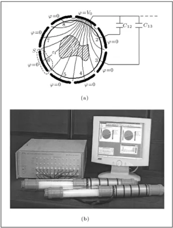
Figure 1 shows a diagram of the ECT measurement (in each scanning, one electrode is at voltage '= V
0 and the others are set to zero volt) and a picture of an experimental ECT system, which includes the electrode array and the shielding.
For the forward problem, a FEM program has been implemented. The forward problem in ECT is an electrostatic problem, where the conductivity is zero and the magnetic eld is neglected. Assuming there are no internal charges, the mathematical model of the
Figure1. (a): A diagram of the ECT sensor and (b): An
8-electrode experimental ECT system for Process Tomography Limited (PTL).
forward problem (for electric potential') is given by: r:("r') = 0; in Vd;
'=vk; on Ek; '= 0; on @Vdn
[
k
Ek; (1)
whereVdis the region the containing the eld (possibly an innite region), "is the dielectric permittivity and Ek is the kth electrode, held at the potential, vk, usually attached on the surface of an insulator. The shields are set to zero volt. The capacitance between excitation and thekth sensing electrode is given by:
C= Q V
0 =
H
S"r':nds V
; (2)
V
0 is the potential dierence between the source and the detecting electrode and Q is the total charge on the measuring electrode. In most practical ECT measurements, the data are normalized as:
Cn=
Cm Cl Ch Cl
; (3)
whereCn is the normalized capacitance between a pair of electrodes, Cm is the measured capacitance andCl and Ch are the capacitances, when the ECT sensor is full of the lower and higher permittivity materials used to calibrate the sensor, respectively. The Finite Element Method (FEM) is used to solve the forward ECT problem [5].
Special attention has been paid to verifying the forward model with experimental data, as the measure-ments of sensor capacitances show that conventional methods for calculating sensitivity matrices can give inaccurate results for pixels close to the electrodes.
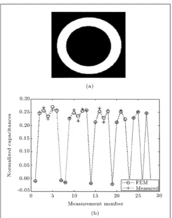
The forward model was veried against an experi-mental test sensor shown in Figure 2. Simulated (FEM) and measured normalized capacitances are shown in Figure 2. The maximum error between the simulated and measured values is less than 0.1%, which is an indication of the accuracy of the forward model for the normalized capacitances. The experimental data was generated by an 8-electrode sensor, 84 mm in diameter. The measurement electrodes are 10 cm long (third direction) mounted symmetrically on the outside of an insulating pipe and 28 measurement data are used. The example considers a single ring of Perspex with a circle in the centre (air with diameter 26 mm) and the fourth example is one circular object (Perspex, 32 mm in diameter) near the wall. All these inclusions are Perspex objects with a relative permittivity of 1.8 and the background is free space with a relative permittivity of 1. The number of
Figure2. (a): A plastic ring with permittivity of 1.8 and
(b): Comparisons of measured and calculated capacitances.
triangular elements are 6400. It should be noted that the accuracy obtained by comparing the measured and calculated absolute capacitances was worse than that for the normalized values. Figure 3b shows the electric potential distribution when electrode 1 was used for the excitation of the empty tank (the FEM mesh showed in Figure 3a). The sensitivity of the change in the measured charges on sensing electrodes to the change of the permittivity of a region in the imaging area is
calculated by (see [4]): dQij
d" "=
Z
"Ei:EjdS; (4)
where Ei and Ej are the electric eld when the exci-tation electrodes are electrodes i and j, respectively, that can be calculated directly from the results of the forward solver. is the perturbation region. Figure 3c shows the sensitivity plot for two opposite electrodes.
IMAGE RECONSTRUCTION
A regularized Gauss-Newton method is a suitable image reconstruction scheme [5,11] for nonlinear ill-posed ECT problems. The image reconstruction is to nd a permittivity map that minimizes:
kCm F(")k 2
+G("); (5)
whereCmincludes the measured capacitances,F(") are the simulated capacitances for the permittivity map,", from the forward problem andG(") is the regulariza-tion term. The most commonly used regularizaregulariza-tion is the Tikhonov regularization [12]. For Tikhonov regularization, the penalty term is:
G(") = Z
jr"j 2
dS: (6)
The forward problem is solved and the measured capacitances compared with the calculated ones from the FE model. The permittivity is then updated using a regularized inverse of the Jacobian. The process is repeated until the predicted capacitances from the nite element method agree with the measured values. The updated formula is:
"n +1=
"n+ (JtnJn+R) 1
Jtn(Cm F("n)); (7)
Figure3. (a): Mesh for the forward problem, (b): Electric potential when electrode 1 is set to 1 volt and the rest of the
where Jn is the Jacobian, calculated with the per-mittivity, "n, Cm is the vector of capacitance mea-surements and the forward solution, F("n), is the predicted capacitance from the FE model. The matrix,
R =
2
LtL, is a regularization matrix, where L is a discrete version of the Laplacian operator and is the regularization parameter, which penalizes extreme changes in permittivity, thus, removing instability in the reconstruction. The regularization parameter, here used empirically ( = 10
5), is the choice for all iterations.
LEVEL SET METHOD
In two-phase material imaging, the goal is to recover information concerning the number, shape, size and, perhaps, contrast of a collection of anomalous regions. There has been growing interest in the development and use of geometrical inversion methods, which move away from the estimation of a dense collection of pixel values and concentrate processing resources directly on the recovery of information regarding anomalies. The problem of the permittivity reconstruction is reformu-lated to a special geometrical representation of the objects. The level set method was initially introduced for tracking the propagating boundaries. In this paper, FEM has been used to solve the forward problem. In order to avoid so-called inverse crime, dierent mesh was used, including a triangular mesh for the FEM model of the forward problem and a grid mesh for level set calculation. With an iterative method and using an update formula for the level set function, an attempt was made to t the measured to the simulated data. A numerical implementation of 2D ECT reconstruction is presented and the results of the shape recovery are promising.
Instead, one can formulate the problem to nd the interface between two materials. The level set technique was chosen to describe the changing shapes, since this method is easily able to model any topological changes in the boundaries.
In the shape reconstruction approach, it is as-sumed that the background distribution and approx-imate values of the image parameter inside the in-clusions are known, but that the number, topology and shape of the obstacles are unknown and have to be recovered from the data. Compared to the more typical pixel-based reconstruction schemes, the shape reconstruction approach has the advantage that the prior information about the high contrast of the inclusions is incorporated explicitly in the modeling of the problem. Although, in a pixel-based reconstruction scheme, the approximate locations of the unknown obstacles are found already during the early iterations, it typically takes a large number of additional iterations in order to actually build up this high contrast to the
background before getting more accurate information concerning the shapes of these objects. This can be done better with a level set approach. Here, the equation describing the moving fronts is:
t+Fjrj= 0; (8)
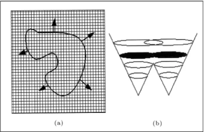
whereF is the speed function and t is the boundary in time t. In Figure 4a, a moving boundary is schematically shown. Figure 4b shows that during the emerging (or separation) of two objects, the same level set function can describe the boundary and that is a major advantage of the level set method.
The describing level set function is a function form,R
2
!R, for this two-dimensional case. Its value is zero in the boundary and it has a negative sign inside and a positive sign outside the boundary.
The permittivity at each point, r, can be de-scribed in terms of the level set function, depending on the position of the point, r, with respect to the boundary,@D, of the inclusion,D, as follows:
"(r) = n
" int
fr;(r)<0g ; "(r) =
n "
ext
fr;(r)>0g;
@D:=fr;(r) = 0g; (9)
here," intand
"
ext are the permittivity of the inclusion and the background, respectively. For a shape-based method, using a level set formulation, the boundaries are moving, in order to reduce mist errors. The method developed in [9,10] is used for the calculation of the gradient for the moving boundaries (change in measured capacitance when an interface is moving between two permittivity regions). In the narrowband level set method, the Jacobian matrix is dened as a narrowband region between two phases. The sensitivity values (change in level set function when an interface
Figure 4. (a): Moving boundary and (b): Emerging
is moving) at each point in the narrowband region is proportional to the dierence between two permittivity values and, also, proportional to term Ei:Ej, a term reecting the sensitivity in permittivity changes. The formulation of Equation 7 with the Jacobian, with respect to the boundary and identity matrix as regular-ization, has been used to update the level set function. The inverse boundary value is to nd a level set function (which, in turn, describes a permittivity distribution) that minimizes the mismatch between the measured and simulated data. The algorithm is as follows:
1. Start with an initial guess for the shape of the inclusion (initial level set function), in this case, a circle located in the centre;
2. Dene the interface and narrow band; the narrow band is an area that includes pixels sharing points with the interface;
3. Solve the forward problem and calculate the Jaco-bian, with respect to the boundary;
4. Update the level set function and calculate a new interface boundary and narrow band;
5. Check the mist in the data; if the error is small enough: Stop;
6. If the mist is not small, go to Step 2.
RESULTS ANDDISCUSSION
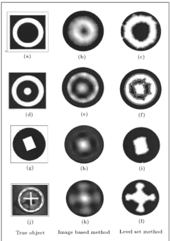
Figure 5 shows the reconstruction of various test ex-amples from an experimental ECT system. On the left hand side, there is a ring, a ring and rod, a rectangular shape and a cross-shaped object. These are the true permittivity; the white color is for a plastic object with a permittivity of 1.8 and the black background is for air. In the middle, there is a reconstruction using an image-based method, namely; a regularized Gauss-Newton method. On the right hand side, the level set based shape reconstruction results are presented. For the image based method, four iterations have been used and the size of the inverse problem is 852 (elements inside the sensor area). The condition number of the image based Jacobian was 2.4e4 (this is based on the Jacobian of the rst step, the initial guess here is free space). For the level set based method, 17, 19, 12 and 21 iterations have been used for test examples of (c), (f), (i) and (l), respectively. The average size of the inverse problem in the level set based method is 325 and the condition number of the Jacobian matrix for the level set based method (rst iteration with the initial guess as a circular of radius 1 cm at the center) is 1.6e3. As expected, the size of the inverse problem, when the narrowband level set method is in use, is smaller and the inverse problem is better conditioned. A smaller sized inverse problem and a
Figure5. Experimental ECT.
better-posed inverse problem are major advantages of the level set method, which enables one to use fewer numbers of measured data. This means that one is unable to use any low quality measurements (for instance, measurement of capacitances in neighboring electrodes).
CONCLUSION
A nonlinear image reconstruction method has been developed and tested using experimental ECT data. The FE based forward solver was also validated using normalized capacitance data. Shape identication in two-phase materials is an inverse boundary value problem; therefore, it is not ecient to use common image reconstruction methods. Shape reconstruction, with real experimental ECT data, is presented in this paper. The main advantage of the level set formulation is that, in each iteration, the inverse problem needs to be solved in the interface between two materials rather than in all regions of interest. In terms of including all prior information, the level set method incorporates important regularization, namely; two-phase material. The level set function could nd the position and a relatively accurate shape of the inclusion; however, more work needs to be done regarding regularization of
this method, in order to improve shape recovery. The result of the level set method is comparable to that of the image based method and the computation time for the shape method is less
REFERENCES
1. Yang, W.Q. and Peng, L.H. \Image reconstruction algorithms for electrical capacitance tomography",
Meas. Sci. Technol. (Review Article), 14, pp R1-R13
(2003).
2. Yang, W.Q. \Calibration of capacitance tomography systems: a new method for setting system measure-ment range", Meas. Sci. Technol., 7, pp L863-L867
(June 1996).
3. Jaworski, A.J. and Dyakowski, T. \Application of electrical capacitance tomography for gas-solids ow",
Measurement Science&Technology,12, pp 1109-1120
(2001).
4. Dyakowski, T., Jeanmeure, L.F.C. and Jaworski, A.J. \Applications of electrical tomography for gas-solids and liquid-solids ows-a review",Powder Technology,
112, pp 174-192, Jonathan Seville, Eleseviere (2000).
5. Soleimani, M. \Image and shape reconstruction for electrical impedance and magnetic induction tomogra-phy", PhD Thesis, University of Manchester (formerly UMIST) (2005).
6. Tamburrino, A., Rubinacci, G., Soleimani, M. and Lionheart, W.R.B. \Non iterative inversion method for electrical resistance, capacitance and inductance
tomography for two phase materials", Proceedings of the 3rd World Congress on Industrial Process Tomog-raphy, Ban, Canada, pp 233-238 (2003).
7. Chung, E.T., Chan, T.F. and Tai, X.C. \Electrical impedance tomography using level set representation and total variational regularization",Journal of Com-putational Physics,205, pp 357-372 (2005).
8. Tai, X.C. and Chan, T.F. \A survey on multiple level set methods with applications for identifying piecewise constant functions", International J. Numer. Anal. Modeling,1(1), pp 25-48 (2004).
9. Dorn, O., Miller, E.L. and Rappaport, C.M. \A shape reconstruction method for electromagnetic to-mography using adjoint elds and level sets", Inverse Problems,16, pp 1119-1156 (2000).
10. Santosa, D.F. \A level-set approach for inverse prob-lems involving obstacles ESAIM: Control", Optimiza-tion and Calculus of VariaOptimiza-tions,1, pp 17-33 (1996).
11. Yang, W.Q., Spink, D.M., York, T.A. and McCann, H. \An image-reconstruction algorithm based on Landwe-ber's iteration method for electrical-capacitance to-mography", Meas. Sci. Technol., 10, pp 1065-1069
(1999).
12. Lionheart, W.R.B. \Reconstruction algorithms for permittivity and conductivity imaging",Proceedings of the 2nd World Congress on Industrial Process Tomog-raphy, Hannover, Germany, 29th-31st August, pp 4-10 (2001).