ITP-UU-09/11 SPIN-09/11
INTRODUCTION TO THE
THEORY OF BLACK HOLES
∗Gerard ’t Hooft
Institute for Theoretical Physics Utrecht University
and
Spinoza Institute Postbox 80.195
3508 TD Utrecht, the Netherlands e-mail: [email protected]
internet: http://www.phys.uu.nl/~thooft/
Version June 9, 2009
Contents
1 Introduction 2
2 The Metric of Space and Time 4
3 Curved coordinates 5
4 A short introduction to General Relativity 6
5 Gravity 9
6 The Schwarzschild Solution 10
7 The Chandrasekhar Limit 13
8 Gravitational Collapse 14
9 The Reissner-Nordstr¨om Solution 18
10 Horizons 20
11 The Kerr and Kerr-Newman Solution 22
12 Penrose diagrams 23
13 Trapped Surfaces 25
14 The four laws of black hole dynamics 29
15 Rindler space-time 31
16 Euclidean gravity 32
17 The Unruh effect 34
18 Hawking radiation 38
19 The implication of black holes for a quantum theory of gravity 40
21 History 47
1.
Introduction
According to Newton’s theory of gravity, the escape velocity v from a distance r from the center of gravity of a heavy object with mass m, is described by
1 2v
2 = G m
r . (1.1)
What happens if a body with a large mass m is compressed so much that the escape velocity from its surface would exceed that of light, or, v > c? Are there bodies with a mass m and radius R such that
2G m
R c2 ≥1 ? (1.2)
This question was asked as early as 1783 by John Mitchell. The situation was investigated further by Pierre Simon de Laplace in 1796. Do rays of light fall back towards the surface of such an object? One would expect that even light cannot escape to infinity. Later, it was suspected that, due to the wave nature of light, it might be able to escape anyway.
Now, we know that such simple considerations are misleading. To understand what happens with such extremely heavy objects, one has to consider Einstein’s theory of relativity, both Special Relativity and General Relativity, the theory that describes the gravitational field when velocities are generated comparable to that of light.
Soon after Albert Einstein formulated this beautiful theory, it was realized that his equations have solutions in closed form. One naturally first tries to find solutions with maximal symmetry, being the radially symmetric case. Much later, also more general solutions, having less symmetry, were discovered. These solutions, however, showed some features that, at first, were difficult to comprehend. There appeared to be singularities that could not possibly be accepted as physical realities, until it was realized that at least some of these singularities were due only to appearances. Upon closer examination, it was discovered what their true physical nature is. It turned out that, at least in principle, a space traveller could go all the way in such a “thing” but never return. Indeed, also light would not emerge out of the central region of these solutions. It was John Archibald Wheeler who dubbed these strange objects “black holes”.
Einstein was not pleased. Like many at first, he believed that these peculiar features were due to bad, or at least incomplete, physical understanding. Surely, he thought, those crazy black holes would go away. Today, however, his equations are much better understood. We not only accept the existence of black holes, we also understand how they can actually form under various circumstances. Theory allows us to calculate the
behavior of material particles, fields or other substances near or inside a black hole. What is more, astronomers have now identified numerous objects in the heavens that completely match the detailed descriptions theoreticians have derived. These objects cannot be interpreted as anything else but black holes. The “astronomical black holes” exhibit no clash whatsoever with other physical laws. Indeed, they have become rich sources of knowledge about physical phenomena under extreme conditions. General Relativity itself can also now be examined up to great accuracies.
Astronomers found that black holes can only form from normal stellar objects if these represent a minimal amount of mass, being several times the mass of the Sun. For low mass black holes, no credible formation process is known, and indeed no indications have been found that black holes much lighter than this “Chandrasekhar limit” exist anywhere in the Universe.
Does this mean that much lighter black holes cannot exist? It is here that one could wonder about all those fundamental assumptions that underly the theory of quantum mechanics, which is the basic framework on which all atomic and sub-atomic processes known appear to be based. Quantum mechanics relies on the assumption that every
physically allowed configuration must be included as taking part in a quantum process.
Failure to take these into account would necessarily lead to inconsistent results. Mini black holes are certainly physically allowed, even if we do not know how they can be formed in practice. They can be formed in principle. Therefore, theoretical physicists have sought for ways to describe these, and in particular they attempted to include them in the general picture of the quantum mechanical interactions that occur in the sub-atomic world.
This turned out not to be easy at all. A remarkable piece of insight was obtained by Stephen Hawking, who did an elementary mental exercise: how should one describe relativistic quantized fields in the vicinity of a black hole? His conclusion was astonishing. He found that the distinction between particles and antiparticles goes awry. Different ob-servers will observe particles in different ways. The only way one could reconcile this with common sense was to accept the conclusion that black holes actually do emit particles, as soon as their Compton wavelengths approach the dimensions of the black hole itself. This so-called “Hawking radiation” would be a property that all black holes have in common, though for the astronomical black holes it would be far too weak to be observed directly. The radiation is purely thermal. The Hawking temperature of a black hole is such that the Wien wave length corresponds to the radius of the black hole itself.
We assume basic knowledge of Special Relativity, assuming c= 1 for our unit system nearly everywhere, and in particular in the last parts of these notes also Quantum Mechan-ics and a basic understanding at an elementary level of Relativistic Quantum Field Theory are assumed. It was my intention not to assume that students have detailed knowledge of General Relativity, and most of these lectures should be understandable without knowing too much General Relativity. However, when it comes to discussing curved coordinates, Section 3, I do need all basic ingredients of that theory, so it is strongly advised to famil-iarize oneself with its basic concepts. The student is advised to consult my lecture notes “Introduction to General Relativity”, http://www.phys.uu.nl/ thooft/lectures/genrel.pdf
whenever something appears to become incomprehensible. Of course, there are numerous other texts on General Relativity; note that there are all sorts of variations in notation used.
2.
The Metric of Space and Time
Points in three-dimensional space are denoted by a triplet of coordinates, ~x = (x, y, z) , which we write as (x1, x2, x3) , and the time at which an event takes place is indicated by a fourth coordinate t = x0/c, where c is the speed of light. The theory of Special Relativity is based on the assumption that all laws of Nature are invariant under a special set of transformations of space and time:
t0 x0 y0 z0 = a0
0 a01 a02 a03
a1
0 a11 a12 a13
a2
0 a21 a22 a23
a3
0 a31 a32 a33 t x y z ,
or xµ0 = X
ν=0,···,3
aµ
νxν , or x0 =A x , (2.1)
provided that the matrix A is such that a special quantity remains invariant:
−c2t02+x02+y02+z02 =−c2t2+x2+y2+z2 ; (2.2) which we also write as:
X
µ,ν=0,···,3
gµνxµxν is invariant, gµν =
−1 0 0 0
0 1 0 0
0 0 1 0
0 0 0 1
. (2.3)
A matrix A with this property is called a Lorentz transformation. The invariance is Lorentz invariance. Usually, we also demand that
a0
0 >0 , det(A) = +1 , (2.4)
in which case we speak of special Lorentz transformations. The special Lorentz transfor-mations form a group called SO(3,1) .
In what follows, summation convention will be used: in every term of an equation where an index such as the index ν in Eqs. (2.1) and (2.3) occurs exactly once as a superscript and once as a subscript, this index will be summed over the values 0,· · ·,3 , so that the summation sign, P, does not have to be indicated explicitly anymore: xµ0 =
aµ
νxν and s2 = gµνxµxν. In the latter expression, summation convention has been
implied twice.
More general linear transformations will turn out to be useful as well, but then (2.2) will not be invariant. In that case, we simply have to replace gµν by an other quantity,
as follows:
so that the expression
s2 =gµνxµxν =gµν0 xµ0xν0 (2.6)
remains obviously valid. Thus, Nature is invariant under general linear transformations provided that we use the transformation rule (2.5) for the tensor gµν. This tensor will
then be more general than (2.3). It is called the metric tensor. The quantity s defined by Eq. (2.6) is assumed to be positive (when the vector is spacelike), i times a positive number (when the vector is timelike), or zero (when xµ is lightlike). It is then called the
invariant length of a Lorentz vector xµ.
In the general coordinate frame, one has to distinguish co-vectors xµ from contra
-vectors xµ. they are related by
xµ=gµνxν ; xµ=gµνxν , (2.7)
where gµν is the inverse of the metric tensor matrix g
µν. Usually, they are denoted by
the same symbol; in a vector or tensor, replacing a subscript index by a superscript index means that, tacitly, it is multiplied by the metric tensor or its inverse, as in Eqs. (2.7).
3.
Curved coordinates
The coordinates used in the previous section are such that they can be used directly to measure, or define, distances and time spans. We will call them Cartesian coordinates. Now consider just any coordinate frame, that is, the original coordinates (t, x, y, z) are completely arbitrary, in general mutually independent, differentiable functions of four quantities u = {uµ, µ = 0,· · ·,3}. Being differentiable here means that every point is
surrounded by a small region where these functions are to a good approximation linear. There, the formalism described in the previous section applies. More precisely, at a given point x in space and time, consider points x+ dx, separated from x by only an infinitesimal distance dx. Then we define ds by
ds2 =gµνdxµdxν =gµν0 (u) duµduν . (3.1)
The prime was written to remind us that gµν in the u coordinates is a different function
than in the x coordinates, but in later sections this will be obvious and we omit the prime. Under a coordinate transformation, gµν transforms as Eq. (2.5), but now these
coefficients are also coodinate dependent:
gµν0 (u) = ∂x
α ∂uµ
∂xβ
∂uν gαβ(x) . (3.2)
In the original, Cartesian coordinates, a particle on which no force acts, will go along a straight line, which we can describe as
dxµ(τ)
dτ =v
µ= constant; vµvµ=−1 ; d2xµ(τ)
y
x
x
′
y
′
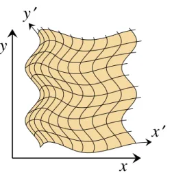
Figure 1: A transition from one coordinate frame {x, y} to an other, curved coordinate frame {x0, y0}.
where τ is the eigen time of the particle. In terms of curved coordinates uµ(x) , this no
longer holds. Suppose that xµ are arbitrary differentiable functions of coordinates uλ.
Then
dxµ
dτ = ∂xµ ∂uλ
duλ
dt ;
d2xµ
dτ2 =
∂2xµ ∂uλ∂uκ
duκ
dτ
duλ
dτ + ∂xµ ∂uλ
d2uλ
dτ2 . (3.4)
Therefore, eq. (3.3) is then replaced by an equation of the form
g0
µν(u)
duµ
dτ
duν
dτ =−1 ;
d2uµ(τ)
dτ2 + Γ
µ
κλ(u)
duκ
dτ
duλ
dτ = 0 , (3.5)
where the function Γµκλ(u) is given by Γµκλ(u) = ∂u
µ ∂xα
∂2xα
∂uκ∂uλ . (3.6)
Here, it was used that partial derivatives are invertible:
∂uµ ∂xα
∂xα ∂uκ
=δα
κ . (3.7)
Γµκλ is called the connection field. Note that it is symmetric under interchange of its two subscript indices:
Γµκλ= Γµλκ . (3.8)
4.
A short introduction to General Relativity
• Ascalar function φ(x) of some arbitrary curved set of coordinates xµ, ia a function
that keeps the same values upon any coordinate transformation. Thus, a coordinate transformation xµ → uλ implies that φ(x) = φ0(u(x)) , where φ0(u) is the same
scalar function, but written in terms of the new coordinates uλ. Usually, we will
• A co-vector is any vectorial function Aα(x) of the curved coordinates xµ that,
upon a curved coordinate transformation, transforms just as the gradient of a scalar function φ(x) . Thus, upon a coordinate transformation, this vectorial function transforms as
Aα(x) = ∂uλ
∂xαAλ(u). (4.1)
.
• A contra-vector Bµ(x) transforms with the inverse of that matrix, or
Bµ(x) = ∂x
µ ∂uλB
λ(u) . (4.2)
This ensures that the product Aα(x)Bα(x) transforms as a scalar: Aα(x)Bα(x) =
∂uλ ∂xα
∂xα
∂uκAλ(u)B
κ(u) =A
λ(u)Bλ(u), (4.3)
where Eq. (3.7) was used.
• A tensor A β1β2···
α1α2··· (x) is a function that transforms just as the product of covectors
A1
α1, A2α2, · · ·, and covectors B1β1, Bβ22 , · · ·. Superscript indices always refer to the contravector transformation rule and subscript indices to the covector transforma-tion rule.
The gradient of a vector or tensor, in general, does not transform as a vector or tensor.
To obtain a quantity that does transform as a true tensor, one must replace the gradient
∂/∂xµ by the so-called the covariant derivative D
µ, which for covectors is defined as DµAλ(x) =
∂Aλ(x) ∂xµ −Γ
ν
µλ(x)Aν(x), (4.4)
for contravectors:
DµBκ(x) =
∂Bκ(x) ∂xµ + Γ
κ
µν(x)Bν(x) , (4.5)
and for tensors:
DµAα1α2β1β2······(x) =
∂ ∂xµA
β1β2···
α1α2··· (x) − Γνµα1(x)Aνα2β1β2··· ···(x)−Γνµα2(x)Aα1νβ1β2··· ···(x)− · · ·
+ Γβ1
µν(x)Aα1α2νβ2······(x) +· · · . (4.6)
In these expressions, Γν
µλ is the connection field that we introduced in Eq. (3.6); there,
however, we assumed a flat coordinate frame to exist. Now, this might not be so. In that case, we use the metric tensor gµν(x) to define Γνµλ. It goes as follows. If we had a flat
coordinate frame, the metric tensor gµν would be constant, so that its gradient vanishes.
Suppose that we demand the covariant derivative of gµν to vanish as well. We have Dµgαβ = ∂
∂xµgαβ −Γ ν
µαgνβ−Γνµβgαν . (4.7)
Lowering indices using the metric tensor, this can be written as
Dµgαβ = ∂
∂xµgαβ−Γβµα−Γαµβ . (4.8)
Taking his covariant derivative to vanish, and using the fact that Γ is symmetric in its last two indices, we derive
Γµκλ = 1
2gµα(∂κgαλ+∂λgακ −∂αgκλ), (4.9) where gµα is the inverse of g
µν, that is,gνµgµα=δνα, and ∂κ stands short for the partial
derivative: ∂κ =∂/∂uκ.
Eq. (4.9) will now be used as a definition of the connection field Γ . Note that it is always symmetric in its two subscript indices:
Γµκλ= Γν
λκ . (4.10)
This definition implies that Dµgαβ = 0 automatically, as an easy calculation shows, and
that the covariant derivatives of all vectors and tensors again transform as vectors and tensors.
It is important to note that the connection field Γα
αβ itself does not transform as a
tensor; indeed, it is designed to fix quantities that aren’t tensors back into forms that are. However, there does exist a quantity that is constructed out of the connection field that does transform as a tensor. This is the so-called Riemann curvature. This object will be used to describe to what extent space-time deviates from being flat. It is a tensor with four indices, defined as follows:
Rµκαβ =∂αΓµκβ−∂βΓµκα+ ΓµασΓσκβ −ΓµβσΓσκα ; (4.11)
in the last two terms, the index σ is summed over, as dictated by the summation con-vention. In the lecture course on general Relativity, the following statement is derived:
If V is a simply connected region in space-time, then the Riemann curvature
Rµκαβ = 0 everywhere in V , if and only if a flat coordinate frame exists in V ,
that is, a coordinate frame in terms of which gµν(x) = gµν0 everywhere in V .
The Ricci curvature is a two-index tensor defined by contracting the Riemann curvature:
Rκα =Rµκµα . (4.12)
The Ricci scalar R is defined by contracting this once again, but because there are only two subscript indices, this contraction must go with the inverse metric tensor:
With some effort, one can derive that the Riemann tensor obeys the following (partial) differential equations, called Bianchi identity:
DαRµκβγ+DβRµκγα+DγRµκαβ = 0 . (4.14)
From that, we derive that the Ricci tensor obeys
gµνD
µRνα−12DαR= 0 . (4.15)
5.
Gravity
Consider a coordinate frame {xµ} where g
µν is time independent: ∂0gµν = 0 , and a
particle that, at one instant, is at rest in this coordinate frame: dxµ/dτ = (1,0,0,0) .
Then, according to Eq. (3.5), it will undergo an acceleration d2xi
dτ2 =−Γ
i
00= 12g
ij∂
jg00 . (5.1)
Since this acceleration is independent of the particle’s mass, this is a perfect description of a gravitational force. In that case, −1
2g00 can serve as an expression for the gravitational
potential (note that, usually, g00 is negative). This is how the use of curved coordinates
can serve as a description of gravity – in particular there must be curvature in the time dependence.
From here it is a small step to think of a space-time where the metric gµν(x) can
be any differentiable function of the coordinates x. Coordinates x in terms of which
gµν is completely constant do not have to exist. The gravitational field of the Earth, for
instance, can be modelled by choosing g00(x) to take the shape of the Earth’s gravitational potential. We then use Eqs. (3.5) and (4.9) to describe the motion of objects in free fall. This is the subject of the discipline called General Relativity.
Of course, no coordinate frame exists in which all objects on or near the Earth move in straight lines, and therefore we expect the Riemann curvature not to vanish. Indeed, we need to have equations that determine the connection field surrounding a heavy object like the Earth such that it describes the gravitational field correctly. In addition, we wish these equations to be invariant under Lorentz transformations. This is achieved if the equations can be written entirely in terms of vectors and tensors, i.e. all terms in the equations must transform as such under coordinate transformations. The gravitational equivalence principle requires that they transform as such underall (differentiable) curved coordinate transformations.
Clearly, the mass density, or equivalently, energy density %(~x, t) must play the role as a source. However, it is the 00 component of a tensor Tµν(x) , the mass-energy-momentum
distribution of matter. So, this tensor must act as the source of the gravitational field. Einstein managed to figure out the correct equations that determine how this matter distribution produces a gravitational field. Tµν(x) is defined such that in flat space-time
(with c = 1 ), T0
flow, which equals themomentum density, and Tij is thetension; for a gas or liquid with
pressure p, the tension is Tij =−p δij. Thecontinuity equation in flat, local coordinates
is
∂iTiµ−∂0T0µ= 0 , µ= 0,1,2,3. (5.2)
Under general coordinate transformations, Tµν transforms as a tensor, just as gµν does,
see Eq. (3.2).
In curved coordinates, or in a gravitational field, the energy-momentum tensor does not obey the continuity equation (5.2), but instead:
gµνD
µTνα = 0 , (5.3)
So, the partial derivative ∂µ has been replaced by the covariant derivative. This means
that there is an extra term containing the connection field Γλ
αβ. This is the gravitational
field, which adds or removes energy and momentum to matter. Einstein’s field equation now reads:
Rµν− 12R gµν =−8πG Tµν , (5.4)
where G is Newton’s constant. The second term in this equation is crucial. In his first attempts to write an equation, Einstein did not have this term, but then he hit upon inconsistencies: there were more equations than unknowns, and they were, in general, conflicting. Now we know the importance of the equation for energy-momentum conser-vation (5.3), written more compactly as DµTνµ = 0 . It matches precisely the Bianchi
identity (4.15) for the Ricci tensor, because that can also be written as
gµνD
µ(Rνα− 12Rgνα) = 0 . (5.5)
6.
The Schwarzschild Solution
When Einstein found his equation, Eq. (5.4), end of 1915, he quickly derived approximate solutions, in order to see its consequences for observations, so that Eddington could set up his expedition to check the deflection of star light by the gravitational field of the sun. Einstein, however, did not expect that the equation could be solved exactly. It was Karl Schwarzschild, in 1916, who discovered that an exact, quite non-trivial solution can be found. We will here skip the details of its derivation, which is straightforward, though somewhat elaborate, and we will see more of that later. Schwarzschild’s description of the metric gµν(x) that solves Einstein’s equations is most easily expressed in the modern
notation:
ds2 =gµνdxµdxν = −(1−2M/r) dt2+ dr
2
1−2M/r+r
2dΩ2 , (6.1)
where Newton’s constant G has been absorbed in the definition of the mass parameter1:
M = Gm. The advantage of this notation is that one can read off easily what the metric looks like if we make a coordinate transformation: just remember that dxµ is an
infinitesimal displacement of a point in space and time. Notice from the dependence on dx02, that indeed, −1
2g00 is the gravitational potential −M/r, apart from the constant 1.
Like other researchers in the early days, Schwarzschild himself was very puzzled by the singularity at r = 2M. He decided to replace the coordinate r by a “better” radial coordinate, let’s call it ˜r, defined as ˜r= (r3−(2M)3)1/3. The reason for this substitution was that Schwarzschild used simplified equations that only hold if the space-time-volume element, det(gµν) =−1 , and the shift he used simply subtracts an amount (2M)3 from
the space-time volume enclosed by r. Now, the singularity occurs at the “origin”, ˜r= 0 . Schwarzschild died only months after his paper was published. His solution is now famous, but the substitution r→r˜ (in the paper, the notation is different) was unnecessary. The apparent singularity at r = 2M is easier to describe when it is kept right where it is, though indeed, we can use any coordinate frame we like to describe this metric. We emphasize that, whether or not the singularity is moved to the origin, only depends on the coordinate frame used, and has no physical significance whatsoever.2
One elegant coordinate substitution is the replacement of r and t by the
Kruskal-Szekeres coordinates x and y, which are defined by the following two equations:
x y = ³ r
2M −1
´
er/(2M) , (6.3)
x/y = et/(2M) . (6.4)
The angular coordinates θ and ϕ are kept the same. By taking the log of Eq. (6.3) and (6.4), and partially differentiating with respect to x and y, we read off:
dx x +
dy
y =
dr r−2M +
dr
2M =
dr
2M(1−2M/r) , (6.5) dx
x −
dy
y =
dt
2M . (6.6)
The Schwarzschild metric is now given by ds2 = 16M2
µ
1− 2M
r
¶ dxdy
x y +r
2dΩ2 = 32M
3
r e
−r/(2M)dxdy+r2dΩ2 . (6.7) Notice now that, in the last expression, the zero and the pole at r = 2M have cancelled out. The function r(x, y) can be obtained by inverting the algebraic expression
1throughout these notes, we will denote the total mass of an object by m, and use the symbol M
for Gm.
2There are some heated discussions of this on weblogs of amateur physicists who did not grab this
0 2M
t
r
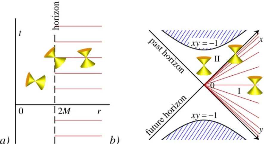
horizon
y x xy = −1
future horizon past horizon
xy = −1
ΙΙ Ι 0
b)
a)
Figure 2: a) The black hole in the Schwarzschild coordinates r, t. The horizon is at r = 2M. b) Kruskal-Szekeres coordinates; here, the coordinates of the horizon are at x= 0 and at y = 0 . The orientation of the local lightcones is indicated. Thin red lines are the time = Constant limes in the physical part of space-time.
(6.3) and is regular in the entire region x y >−1 . In particular, nothing special seems to happen on the two lines x = 0 and y = 0 . Apparently, there is no physical singularity
or curvature singularity at r → 2M. We do notice that the line x = 0, θ and ϕ both
constant, is lightlike, since two neighboring points on that line obey dx= dθ= dϕ= 0 , and this implies that ds = 0 , regardless the value of dy. similarly, the line y = 0 is lightlike. Indeed, we can also read off from the original expression (6.1) that if r= 2M, the lines with constant θ and ϕ are lightlike, as ds = 0 regardless the value of dt. The line y = 0 is called the future horizon and the line x = 0 is the past horizon (see Section 10).
An other important thing to observe is that Eq. (6.4) attaches a real value for the time t when x and y both have the same sign, such as is the case in the region marked
I in Fig. 2b, but if x y <0 , as in region II, the coordinate t gets an imaginary part. This means that region II is not part of our universe. Actually, t does not serve as a time coordinate there, but as a space coordinate, since there, dt2 enters with a positive sign in the metric (6.1). r is then the time coordinate.
Even if we restrict ourselves to the regions where t is real, we find that, in general, every point (r, t) in the physical region of space-time is mapped onto two points in the (x, y) plane: the points (x, y) and (−x,−y) are mapped onto the same point (r, r) . This leads to the picture of a black hole being a wormhole connecting our universe to another universe, or perhaps another region of the space-time of our universe. However, there are no timelike or light like paths connecting these two universes. If this is a wormhole at all, it is a purely spacelike one.
7.
The Chandrasekhar Limit
Consider Einstein’s equation (5.4), and some spherically symmetric, stationary distribu-tion of matter. Let p(r) be the r dependent pressure, and %(r) the r dependent local mass density. An equation of state for the material relates p to %. In terms of an aux-iliary variable m(r) , roughly to be interpreted as the gravitational mass enclosed within a sphere with radius r, and putting c= 1 , one can derive the following equations from General Relativity:
dp
dr = −G
(%+p)(m+ 4πp r3)
r2(1−2Gm/r) , (7.1)
dm
dr = 4π% r
2 . (7.2)
These equations are known as the Tolman-Oppenheimer-Volkoff equations. The last of these, Eq. (7.2) seems to be easy to interpret. The first however, Eq. (7.1), seems to imply that not only energy but also pressure causes gravitational attraction. This is a peculiar consequence of the trace part of Einstein’s equation (5.4). In many cases, such as the calculation of the gravitational forces between stars and planets, the pressure term cancels out precisely. This is when there is a boundary where the pressure vanishes.
The resulting space-time metric is calculated to take the form
ds2 =−A(r)dt2+B(r)dr2+r2(dθ2+ sin2θdϕ2) , (7.3) where
B(r) = 1
1−2Gm(r)/r ; (7.4)
and
log(A(r)B(r)) = −8πG
Z ∞
r
(p+ρ)rdr
1−2Gm(r)/r . (7.5)
Note that the Tolman-Oppenheimer-Volkoff equations (7.1) and (7.2) are exact, as soon as spherical symmetry and time independence are assumed.
There is no stable solution of the Tolman-Oppenheimer-Volkoff equations if, anywhere along the radius r, the enclosed gravitational mass M(r) = Gm(r) exceeds the value
r/2 . If the equation of state allows the pressure to be high while the density % is small, then large amounts of total mass will still show stable solutions, but if we have a liquid that is cool enough to show a fixed energy density %0 even when the pressure is low, the enclosed mass would be approximately 4
3π%0r3, so with sufficiently large quantities of mass you can always exceed that limit. Thus, at sufficiently low temperatures, no stable, non-singular solution can exist if the baryonic mass NB exceeds some critical value.
Integrating inwards, one finds that there will be values of r where M(r)/r exceeds the critical value 1/2 so that A(r) and B(r) develop singularities.
Substituting some realistic equation of state at sufficiently low temperature, one de-rives that the smallest amount of total mass needed to make a black hole is then a little more than one solar mass. The Chandrasekhar limit refers to the largest amount of mass one can make of a substance where only electron pressure resists the gravitational attraction. This limit is about 1.44 solar masses.
One must ask what happens when larger quantities of mass are concentrated in a small enough volume. If no stable solution exists, this must mean that the system collapses under its own weight. What will happen to it?
8.
Gravitational Collapse
An extreme case is matter of the form where the pressure p vanishes everywhere. This is called dust. When at rest, in a local Lorentz frame, dust has only an energy density
T00 =−% while all other components of Tµν vanish. In any other coordinate frame, the
energy-momentum tensor takes the form
Tdustµν =−%(x)vµvν , (8.1)
where vµ is the local velocity dxµ/dτ of the dust grains.
In that case (and if we insist on spherical symmetry, so that the total angular mo-mentum vanishes), gravitational implosion can never be avoided. It is instructive to show some simple exact solutions.
Consider as initial state a large sphere of matter contracting at a certain speed v. We could take v to be anything, but for simplicity we here choose it to be the velocity of light. Thus, at t→ −∞ we take for the energy density T0
0 (and for simplicity G= 1 ),
T00(r, t)→%0δ(r+t)/r2 , (8.2) where the factor r−2 was inserted to ensure conservation of energy at infinity:
E = Z ∞
0
dr4πr2T00(r, t) = 4π%0 . (8.3) Thus, at t→ −∞, matter is assumed to be confined into a thin, dense shell with radius
r→ |t|.
With this initial condition, and the equation of state p= 0 , it is not so difficult simply to guess the exact solution: we assume the metric to be stationary both before and after the passage of the dust shell, but while the dust shell passes there is a jump proportional to a theta step function. Both inside the dust shell and outside, spherical symmetry demands that the only admissible solution will then be the Schwarzschild metric with mass parameter M, however, M outside is different from M inside. With our initial condition (8.2), we have to choose M inside to be zero, but, for future use, we will also consider more general solutions, with different values for Min and Mout. We will have to verify afterwards that the configuration obtained is indeed a correct solution, but we can
already observe that spherical symmetry would not have left us any alternative. What has to be done now is to carefully formulate the matching conditions of the two regions at the location of the contracting dust shell.
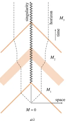
space
singularity
horizon
time
M = 0
M1 M2
M3
b) a)
M = 0 M1 M2 M3
r tcom
Figure 3: Several shells of matter (shaded lines) implode to form a black hole, whose mass M increases. In a) , time is neither the Schwarzschild time nor the tcom coordinate, but it indicates the causal order of events. The dotted line is the location of the horizon. In b) , the coordinates tcom and r are used. The dotted line here is the apparent Schwarzschild horizon r = 2M. Here, 0< M1 < M2 < M3.
The contracting dust shell follows a lightlike geodesic in the radial direction, given by ds2 = 0 , or
dr
dt = −
r
A
B =
2M
r −1 , (8.4)
so that
dt
dr =
−r
r−2M → t(r) =−r−2Mlog(r−2M). (8.5)
This is a reason to use a modified coordinate frame both in the inside region and the out-side region. Inout-side, we use the Schwarzschild metric with coordinates (tin, r, θ, ϕ) , and outside we use (tout, r, θ, ϕ) , but in both regions we make the transition to coordinates
(tcom, r, θ, ϕ) , where
tcom = tin+r+ 2Minlog(r−2Min),
tcom = tout+r+ 2Moutlog(r−2Mout) . (8.6) Remember that for our original problem, Min = 0 , so that, according to the initial condition (8.2), the dust shell moves at the orbit tcom = 0 . We call tcom the co-moving time. tcom=Cst is a geodesic in both regions. The matching condition will now be that at the points tcom = 0 the two regions are stitched together. The coordinates r, θ and
ϕ will be the same for both regions (otherwise the metric gµν would show inadmissible
discontinuities3). At t
com<0 we have M =Min and at tcom>0 we have M =Mout. In terms of the new coordinates, the metric is
ds2 = −A Ã
dt− r
B Adr
!2
+Bdr2 +r2dΩ2 = −Adt2+ 2 dtdr+r2dΩ2
= µ
−1 + µ(t)
r
dt2+ 2 dtdr+r2dΩ2 , (8.7) where
µ(t) = 2M(t), M(t) = θ(t)Mout +θ(−t)Min , (8.8) and we dropped the subscript “com” for the time coordinate t.
In fact, any monotonously rising function µ(t) will be a solution to Einstein’s equa-tions where dust flows inwards with the speed of light. To check the solution now, let us evaluate the Ricci curvature for the metric (8.7) in these coordinates:
g00=−1 +
µ
r , g10=g01 = 1 , g11= 0 , g00 = 0 , g10 =g01= 1 , g11= 1−µ
r ; (8.9)
defining ˙µ= dµ/dt, we find4for the Christoffel symbols, Γ
αµν = 12(∂µgαν+∂νgαµ−∂agµν) ,
Γ000 = ˙
µ
2r , Γ100 = µ
2r2 , Γ010 = Γ001=−
µ
2r2 ; Γ122 =−r , Γ133 =−rsin2θ ,
Γ121 = Γ221 =r , Γ313 = Γ331=rsin2θ ,
Γ233 =−r2sinθcosθ , Γ323 = Γ332=r2sinθcosθ ; (8.10)
3In a space-time where the Ricci tensor is allowed to have a Dirac delta distribution, there must always
be a coordinate frame such that: the second derivatives of the metric gµν may have delta peaks, but
thefirst derivatives have at most discontinuities in the form of step functions, while the metric itself is continuous. If then a coordinate transformation is applied with a discontinuous first derivative, such as x→(a+b θ(y))y, with a >0 and a+b >0 , the metric gxx may show a discontinuity; compare the
discontinuity in g00 as a function of tcom in Eq. (8.9).
4Remember that indices are raised and lowered by multiplying these fields with the metric tensor g µν
Γ0 00=
µ
2r2 , Γ 1
10 = Γ101=−
µ
2r2 , Γ1
00 = ˙
µ
2r + µ
2r2 −
µ2 2r3 , Γ0
22 =−r , Γ033=−rsin2θ , Γ122 =µ−r , Γ133 = (µ−r) sin2θ , Γ2
12 = Γ221 = 1
r , Γ
3
13 = Γ331= cotθ ; √
−g =r2sinθ , log√−g = 2 logr+ logθ . (8.11) Inserting these in the equation for the Ricci curvature,
Rµν =−(log
√
−g),µ,ν+ Γαµν,α−ΓβαµΓαβν+ Γαµν(log
√
−g)α , (8.12)
we find that
R00 = ˙
µ
r2 , (8.13)
while all other components of Rµν in these coordinates vanish. It follows also for the
trace5 that R = 0 , because g00= 0 . Hence
G T00 = −1
8π
˙
µ r2 =
−M˙
4πr2 , (8.14)
while all other components, notably also T11, vanish. To see that this is indeed the energy momentum tensor of our dust shell, we note that, in our co-moving coordinates, the 4-velocity is vµ = (0,−Λ,0,0) , where Λ tends to infinity (our “dust” goes with the
speed of light). From Eq. (8.9), we derive that vµ= (−Λ,0,0,0) , and we have agreement
with Eq. (8.14) if
G %= M˙
4πr2Λ2 . (8.15)
We have
vµ =−Λ∂µtcom , (8.16)
so that, in the original Schwarzschild coordinates, where tcom is replaced by tin or tout, according to Eq. (8.6),
vµ= Λ
µ
−1, −1
1−2M/r, 0, 0
; vµ = Λ
µ 1
1−2M/r, −1, 0, 0
; (8.17) here M is the local mass parameter. From the second expression in Eq. (8.17), we see that indeed the shell is moving inwards, with the local speed of light. The situation is
5The fact that R= 0 ensues from our choice to have the dust move with the speed of light. Of course,
this is a limiting case, where all of the energy of the dust is kinetic, and the rest mass is negligible. The Ricci scalar R refers to this fact, that the dust has negligible rest mass.
sketched in Figures 3a) and b) . One readily finds that, if Min is taken to be zero,
Moutis indeed the total energy E of our initial dust shell, defined while it was still at
r→ ∞, in Eq. (8.3).
With a bit more work, this exercise can be repeated for dust going slower than the speed of light. What we see is that, just behind the first dust shell, the Schwarzschild metric emerges. Subsequent shells of dust go straight through the horizon, generating Schwarzschild metrics with larger mass parameters M. Taking M a continuous function of tcom leads to a description of less singular, spherically symmetric clouds of dust, coalescing to form a black hole.
At this stage it is very important to observe that this description of “gravitational collapse” allows for small perturbations to be added to it. For instance, one might assume a tiny amount of angular momentum or other violations of spherical symmetry in the initial state. This is what we mean when we say that the solution is ‘robust’. The horizon at r= 2M might wobble a bit, but it cannot be removed by small perturbations only. This is because the horizon is not a true singularity but rather an artefact of the coordinates chosen. The singularity at r = 0 on the other hand, is very sensitive to small perturbations, but it does not play a role in the physically observable properties of the black hole; it is well hidden way behind the horizon (an observation called Cosmic
Censorship).
9.
The Reissner-Nordstr¨
om Solution
The Maxwell equations in curved space-time, when written in terms of the antisymmetric, covariant tensor Fµν(x) , are easy to find by replacing partial derivatives by covariant
derivatives:
• The homogeneous Maxwell equation remains the same:
∂αFβγ+∂βFγα+∂γFαβ = 0 , (9.1)
because the contributions of the connection fields cancel out due to the complete antisymmetry under permutations of α, β, and γ. Hence, we still have a vector potential field Aµ obeying
Fµν =∂µAν −∂νAµ . (9.2)
• The inhomogeneous Maxwell equation is now
DµFνµ=gαβDαFβν =−Jν , (9.3)
where Jν(x) is the electro magnetic charge and current distribution. This can be
rewritten as
∂µ(
√
where the quantity g is the determinant of the metric:
g = det
µ,ν(gµν) , (9.5)
so that we have the conservation law
∂µ(
√
−g Jµ) = 0 , (9.6)
because the Maxwell field Fµν is antisymmetric in its two indices.
• The energy momentum distribution of the Maxwell field is
Tµν =−FµαFνα+ (14FαβFαβ −JαAα)gµν . (9.7) Spherical symmetry can still be used as a starting point for the construction of a solution of the combined Einstein-Maxwell equations for the fields surrounding a “planet” with electric charge Q and mass m. Just as Eq. (7.3) we choose
ds2 = −Adt2+Bdr2+r2(dθ2+ sin2θdϕ2), (9.8) but now also a static electric field, defined by Ei(x) =F0i =−Fi0:
Er = E(r) ; Eθ = Eϕ = 0 ; B~ = 0. (9.9)
Let us assume that the source Jµ of this field is inside the planet and we are only
interested in the solution outside the planet. So there we have
Jµ = 0 . (9.10)
Since g = −ABr4sin2θ, and F0r = − 1
ABE(r) , the inhomogeneous Maxwell law (9.4)
implies
∂r
³E(r)r2 √
AB
´
= 0 , (9.11)
and consequently,
E(r) = Q √
AB
4πr2 , (9.12)
where Q is an integration constant, to be identified with electric charge since at r → ∞ both A and B tend to 1 .
The homogeneous parts of Maxwell’s law are automatically obeyed because there is a field A0 (potential field) with
The field (9.12) contributes to Tµν:
T00 = −E2/2B = −AQ2/32π2r4 ; (9.14)
T11 = E2/2A = BQ2/32π2r4 ; (9.15)
T22 = −E2r2/2AB = −Q2/32π2r2 , (9.16)
T33 = T22sin2θ = −Q2sin2θ /32π2r2 . (9.17) We find
Tµ
µ = gµνTµν = 0 ; R = 0, (9.18)
a general property of the free Maxwell field. In this case we have (putting G= 1 )
Rµν = −8π Tµν. (9.19)
Herewith the Einstein equation (5.4) lead to the following solution:
A = 1− 2M
r +
Q2
4πr2 ; B = 1/A . (9.20)
This is the Reissner-Nordstr¨om solution (1916, 1918).
If we choose Q2/4π < M2 there are two “horizons”, the roots of the equation A= 0 :
r = r± = M±
p
M2−Q2/4π . (9.21)
Again these singularities are artifacts of our coordinate choice and can be removed by generalizations of the Kruskal-Szekeres coordinates.
We have not shown the complete derivations of these solutions. In principle, the information given in these notes should suffice to derive them, but if further details are needed we refer to the various more elaborate texts in General Relativity. In these lecture notes we concentrate on the physical properties of the various metrics that were found.
10.
Horizons
Consider the metric (6.1), and a light ray going radially inward. The equation for such a light ray is
ds2 = 0 ; dΩ = 0 , or dt dr =
1
1−2M/r . (10.1)
The solution of this equation is
t =t0±(r+ 2Mlog(r−2M)) , (10.2) where t0 is an integration constant, and we choose the minus sign, so that, at r very close to 2M,
Similarly, a ray going radially outward is given by
r(t)→2M +e(t−t1)/2M−1 . (10.4) Note that neither of these light rays ever pass through the barrier r = 2M. Rays going at an angle rather than radially also will not pass through this point. This is why this point is called a horizon. In general, a horizon forms when the coefficient A in the metric (9.8) tends to zero sufficiently fast.
In terms of the Kruskal coordinates, Eqs. (6.7), the inwards and outwards light rays are easier to find: the in-rays are at x =Cst, and the out-rays at y =Cst, where Cst is any positive constant. In these coordinates, however, we see something new. The light rays do actually cross the horizon. Beyond the horizon, they hit upon the singularity at
xy=−1 , which is the point r = 0 .
In solutions that are more general than the Schwarzschild solution, the horizon is defined to be the boundary line between two regions of space-time. Region I is the region defined by all space-time points x from which a geodesic can start, heading towards the future direction, that reaches the boundary at r = ∞. Region II is the collection of points that have no such geodesics attached to them. This means that particles, or indeed astronauts, cannot reach infinity from these points, regardless the value and direction of their initial velocity. The boundary line between I and II, the horizon, is a surface formed by lightlike geodesics pointing radially outwards.
There is also such a surface of lightlike geodesics pointing inwards. For the Schwarz-schild solution, both horizons are at r = 2GM, but we see in the Kruskal frame that actually, the two horizons do not coincide.
In the Reissner-Nordstr¨om solution, we see that the function A(r) has two zeros. The largest one, at
r =M +pM2 −Q2/4π , (10.5)
coincides with the Schwarzschild horizon in the limit Q→0 . It has the same properties as the Schwarzschild horizon.
The second horizon, at
r=M −pM2−Q2/4π , (10.6)
goes to the singularity r = 0 in the limit Q → 0 . But at finite Q it is also a lightlike surface.
Whatever happens within the horizon might be called physically irrelevant, since in-formation concerning the interior region cannot be sent out using light rays. However, later we will see that quantum effects do depend on details of the horizon region, and to understand these, one may have to pass beyond the horizon.
The true, physical singularity that occurs at r = 0 , is far hidden from observation; this singularity may be compared with singularities in physical equations when some parameters such as the time parameter become complex. Kepler’s elliptical orbits, for instance, show delicate singularities at points in complex time, but the planets in the solar system do not seem to be bothered about that.
11.
The Kerr and Kerr-Newman Solution
A fast rotating planet has a gravitational field that is no longer spherically symmetric but is only symmetric under rotations around the z-axis. We here just give the solution:
ds2 = −dt2+ (r2+a2) sin2θdϕ2+ 2Mr(dt−asin2θdϕ)2
r2+a2cos2θ +(r2+a2cos2θ)³dθ2+ dr2
r2−2Mr+a2 ´
. (11.1)
This solution was found by R. Kerr in 1963. To prove that this is indeed a solution of Einstein’s equations requires patience but is not difficult. For a derivation using more ele-mentary principles more powerful techniques and machinery of mathematical physics are needed. The free parameter a in this solution can be identified with angular momentum:
J =a M . (11.2)
c) The Newman et al solution
For sake of completeness we also mention that rotating planets can also be electrically charged. The solution for that case was found by Newman et al in 1965. The metric is:
ds2 = −∆
Y (dt−asin
2θdϕ)2+sin2θ
Y (adt−(r
2+a2)dϕ)2+ Y ∆dr
2+Ydθ2, (11.3) where
Y = r2+a2cos2θ , (11.4)
∆ = r2−2Mr+Q2/4π+a2 . (11.5) The vector potential is
A0 = −
Qr
4πY ; A3 =
Qrasin2θ
4πY . (11.6)
Eq. (11.2) here also describes the total angular momentum in the solution. The Kerr-Newman solution is the most general stationary solution for a black hole with electric
charge, if no matter is present.
As with the Reissner-Nordstr¨om solution, the zeros of the function ∆(r) ar not true singularities but rather coordinate singularities. The only genuine singularity in the cur-vature of space and time occurs where Y(r, θ) = 0 , but this occurs only when both r
and θ are zero: the singularity liesalong the equator at r = 0 .
Exercise: show that when Q= 0 , Eqs. (11.1) and (11.3) coincide.
Exercise: find the non-rotating magnetic monopole solution by postulating a radial
Exercise: derive the gravitational field for a non-relativistic source by linearizing Einstein’s equation (5.4), and use that to derive Eq. (11.2).
Exercise for the advanced student: describe geodesics in the Kerr solution.
12.
Penrose diagrams
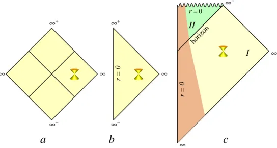
horizon
horizon
xP
yP r = 0 singularity
r = 0 singularity
III II
IV I
∞+
∞−
∞
Figure 4: The Penrose diagram for the Schwarzschild solution
∞ ∞
∞+
∞−
∞
∞− ∞+
r = 0
horizon
r = 0
r = 0
II
I
∞+
∞−
∞
c
b
a
Figure 5: a) Penrose diagram for the Minkowski vacuum with Cartesian transverse coordinates, b) Minkowski space in polar coordinates; c) Penrose diagram for a black hole formed by matter (darker color represents matter falling in).
It is of interest to find coordinate systems that are such that they cover all of space-time that is continuously connected to the region that one has studied before, preferably avoiding any coordinate-induced singularities. This is not always possible, but we can try to choose the best possible coordinates. A good example is the Kruskal-Szekeres
r = r
+
r = r
+
r = r
+
r = r
+
r = 0 singularity
r = 0 singularity
r = r
−
r = r
−
r = r
−
r = r
−
r = r
+
r = r
+
r = r
+
r = r
+
r = 0 singularity
r = 0 singularity
r = r
−
r = r
−
r = r
−
r = r
− VII VI V III II IV I ∞+ ∞− ∞
r = r
+
r = r
+
r = r
+
r = r
+
ring singularity
ring singularity
r = r
−
r = r
−
r = r
−
r = r
−
r = r
+
r = r
+
r = r
+
r = r
+
ring singularity
ring singularity
r = r
−
r = r
−
r = r
−
r = r
− VII VI’ VI V’ V III II IV I ∞+ ∞− ∞ b a
Figure 6: Penrose diagram for the Reissner-Nordstr¨om (a) and the Kerr black hole (b). The singularity at r= 0 is a natural boundary in case of Reissner-Nordstr¨om, but it is a ring singularity in case of Kerr- and Kerr-Newman, through which one can continue to asymptotically flat universes V0 and V I0,
containing a negative mass Kerr Newman black hole.
coordinate system, (6.3) — (6.4), for the Schwarzschild black hole. At every point in the
x y frame of these coordinates, light rays are constrained to form angles of 45◦ or less
with the vertical (vertical meaning the line dx+ dy = 0 ). Or, light rays themselves form trajectories of the form dx≥0, dy ≤0 , where one of the equal signs is reached as soon as dθ = dϕ= 0 .
Now these are not the only coordinates with this property. If the x coordinate is replaces by any monotonously increasing, differentiable function xP of x, and y by any
monotonously increasing differentiable function yP of y, we still have the same property.
This freedom we can use to obtain one other desirable feature: map the point x = ∞ to xP = 1 and the same for y and yP . Furthermore, we can assure that the r = 0
singularity is mapped onto a straight line, here the line xP−yP = 1 . In the Schwarzschild
case, this feature is reached if we choose
Space-time is then sketched in Fig. 4.
A Penrose diagram now is a representation of two of the space-time coordinates in
such a way that the local light cones always show that light rays go with a maximal velocity +1 to the right or -1 to the left, so that the fastest way to transmit information is by rays that are tilted by 45◦ to the left or to the right, such as is the case in Figure
4. The other two coordinates, θ and ϕ usually define a two-sphere. Characteristic boundaries are represented as much as possible by straight lines, which is usually possible and has the advantage that the entire space-time can be represented in a finite patch of the coordinates.
The diagram of Fig. 4 shows four regions of space-time, separated by horizons. Region
I is the region that can be reached from infinity and from which one can also escape to infinity. Region II is the domain behind the horizon that can be reached by test objects falling in, but from where no escape back to infinity is possible. The r = 0 singularity lies in the future of any test object there. Region III is a domain that cannot be reached from infinity, but escape to infinity is allowed. Finally, region IV is only connected to the physical spacetime I by spacelike geodesics.
The Penrose diagram of flat Minkowski space-time is shown in Figure 5a. Figure 5b
describes a black hole formed by matter. We see that at negative times it corresponds to that of Minkowski space-time. At early times, the point r = 0 in 3-space forms a timelike geodesic; at later times it becomes spacelike
13.
Trapped Surfaces
A black hole is characterized by the presence of a region in space-time from which no trajectories can be found that escape to infinity while keeping a velocity smaller than that of light. This implies the presence of trapped surfaces there. We start from the following definitions.
Consider a two-dimensional, closed, convex, spacelike surface S in a curved space-time. Let A be the surface area of S (calculated using the induced metric on S. Define a time coordinate t such that t= 0 on that surface. Suppose that our surface at t = 0 divides 3-space into two regions: an outer region V1 and an inner region V2. A small instant later, at time t =ε, 3-space is divided in three regions:
– an outer region V1 that is spacelike separated from S,
– an inner region V2 that is also spacelike separated from S, and
– a region V3 between V1 and V2 that can be reached by timelike geodesics from S. Its boundary can be reached with lightlike geodesics from S.
Let S1 be the boundary between V1 and V3 and S2 be the boundary between V2 and
S
V
V
3V
2V
1S
2S
1Figure 7: A surface S at t = 0 as described in the text. A little later, at
t = ε, signals moving inwards and outwards divide 3-space into the regions
V1, V2 and V3.
expansion rates θ1, θ2 of these two surfaces as follows:
θ1 = dA1
dε , θ2 =
dA2
dε . (13.1)
Under non-exotic circumstances, such as in a flat space-time, certainly the outer surface expansion rate is positive: θ1 >0 . The inner one is usually negative. However, inside a black hole, we can have a trapped surface. S is called trapped iff both expansion rates are negative or zero:
θ1 ≤0 and θ2 ≤0. (13.2)
A surface ismarginally trapped if the equal sign in Eq. (13.2) holds. For a pure Schwarz-schild black hole, the surface r= 2M is marginally trapped. This is because all light-like geodesics leaving this surface have r = 2M, so that its area, which in the local induced metric is 4π(2M)2, does not increase with time.
What happens in the presence of matter, when the solutions of Einstein’s equations look a lot more complicated? In that case, we can still define trapped surfaces, and they obey a number of important theorems. One of the most important theorems is:
If, in all locally regular coordinate frames, the matter distribution in a space-time obeys the constraint that the energy density is non-negative anywhere, or, in our notation,
T00 ≤0 (13.3)
in all coordinate frames, then
- a trapped surface stays trapped forever, and
- the area of the largest trapped surface can only stay constant or increase. The importance of this theorem is that it shows that black holes cannot disappear once they have been formed.6 Indeed, other theorems show the inevitability of singularities
6Of course, we have not yet considered quantum mechanical effects. These can indeed cause black