Proceedings of the
7th International Workshop on Graph Based Tools
(GraBaTs 2012)
Rooted Graph Programs
Christopher Bak and Detlef Plump
12 pages
Guest Editors: Christian Krause, Bernhard Westfechtel
Managing Editors: Tiziana Margaria, Julia Padberg, Gabriele Taentzer
Rooted Graph Programs
Christopher Bak and Detlef Plump
The University of York, UK
Abstract:We present an approach for programming with graph transformation rules in which programs can be as efficient as programs in imperative languages. The ba-sic idea is to equip rules and host graphs with distinguished nodes, so-called roots, and to match roots in rules with roots in host graphs. This enables graph transforma-tion rules to be matched in constant time, provided that host graphs have a bounded node degree (which in practice is often the case). Hence, for example, programs with a linear bound on the number of rule applications run in truly linear time. We demonstrate the feasibility of this approach with a case study in graph colouring.
Keywords: Graph programs, rooted graphs, time complexity, constant-time graph matching, graph colouring
1
Introduction
The bottleneck for using graph transformation rules in programming is the inefficiency of graph matching. In general, to match the left-hand graphL of a rule within a host graphGrequires time size(G)size(L). As a consequence, linear graph algorithms are slowed down to polynomial complexity when they are recast as programmed graph transformation systems.
One way to speed up graph matching, going back to D¨orr [5], is to equip rules and host graphs with distinguished nodes, so-called roots, and to match roots in rules with roots in host graphs. The same idea underlies Fujaba’s requirement that each method must have a “this” node at which graph matching starts [8,12]. A related concept in GrGen are rules that return graph elements to restrict the location of subsequent rule applications [6].
Dodds and Plump [4,2] have considered rooted graph transformation by using uniquely la-belled nodes as roots. They show that graph matching can be achieved in constant time if rules have a connected left-hand graph and host graphs have bounded node degrees. In addition, they use rooted rules in a rule-based extension of C that allows to check the shape safety of pointer manipulations [3]. In this paper, we generalise the approach of [4,2] from plain rules to pro-grams in the graph programming language GP 2 [10]. We extend GP with rooted rule schemata and present a matching algorithm which deals with the label expressions in these schemata.
of input graphs, demonstrating that rooted GP programs can achieve the time complexity of programs in imperative languages.
2
Graph Transformation
We first recall the graph transformation approach underlying GP, namely the double-pushout approach with relabelling [7], and then accommodate this framework to rooted graphs.
2.1 Non-rooted graph transformation
A (partially labelled) graph Gis a systemG=hVG,EG,sG,tG,lG,mGi whereVG is a finite set ofnodes, EGis a finite set of edges,sGandtG are functions that assign to each edge a source and a target node respectively,lGis the partial node-labelling function andmGis the total edge-labelling function. We writelG=⊥iflG(v)is undefined. Both node and edge labels are taken from a fixed label setL. Unlabelled nodes are used in rules to relabel nodes (see below). There is no need to relabel edges because they can be deleted and reinserted with a new label.
A node w is reachable from a node v if v=w or there are an edge e and a node v0 such thatv andv0 are incident to e and wis reachable from v0. (Note that this defines undirected reachability.) An edgeeis reachable fromvif the source and target ofeare reachable fromv. A graph isconnectedif every node is reachable from every other node.
Given graphsG andH, a premorphism g: G→H is a pair of functions gV:VG→VH and gE: EG→EH that preserve sources and targets. That is, for all edges e in G, sH(gE(e)) = gV(sG(e))and tH(gE(e)) =gV(tG(e)). Ifg also preserves labels, that is mH(gE(e)) =mG(e) for all edgese andlH(gV(v)) =lG(v) for all nodesvwithlG(v)6=⊥, thengis a morphism. A morphism whose node and edge functions are both injective and surjective is anisomorphism. If gsatisfiesg(x) =xfor all nodes and edgesx, thengis aninclusion.
Arule r=hL←K→Riis a pair of inclusionsK→LandK→RwhereLandRare totally labelled graphs. We refer toL,RandKas theleft-hand side, theright-hand sideand theinterface, respectively.
Given a graphGand a ruler=hL←K→Ri, an injective morphismg:L→Gsatisfies the dangling conditionif no node ing(L)−g(K)is incident to an edge inG−g(L). In this caseG directly derivesgraphH, denoted byG⇒r,gHor justG⇒rH, ifH can be constructed fromG as follows:
1. Obtain a subgraphDby removing all nodes and edges ing(L)−g(K).
2. Add (disjointly) the nodes and edges of R−K to D, keeping all labels. For e∈ER− EK, sH(e) =sR(e)ifsR(e)∈VR−VK, otherwise sH(e) =gV(sR(e)). Targets are defined analogously.
3. For allv∈VKwithlK(v) =⊥, definelH(gV(v)) =lR(v). The resulting graph is H.
2.2 Rooted graph transformation
We extend the above definitions to include distinguished root nodes in both rules and host graphs. Our approach is to treat rooted graphs and root-preserving morphisms as “first-class citizens” instead of encoding roots with labels. Unlike [4,2], we allow multiple roots in rule schemata and host graphs; this may be useful in applications with disconnected host graphs.
Arooted graphis a pairhG,PGiwhereGis a graph andPG⊆VGis a set ofroots. A morphism g:G→H isroot-preserving ifg(PG)⊆PH. Note that rooted graphs (over some label set) and root-preserving morphisms form a category.
Arooted rule r=hhL,PLi ← hK,PKi → hR,PRiiis a pair of root-preserving inclusionshK,PKi →
hL,PLiandhK,PKi → hR,PRiwhereLandRare totally labelled. Given a rooted graphGand a root-preserving injective morphismg:L→Gsatisfying the dangling condition, a direct deriva-tionG⇒r,gHis constructed as above and by definingPH= (PG−gV(PL−PK))∪(PR−PK). This construction can be characterised by a pair of natural pushouts in the category of rooted graphs and root-preserving morphisms (omitted for lack of space).
3
Rooted Graph Programs in GP
We extend the graph programming language GP with rooted programs. A complete definition of GP and its revised version GP 2 is given in [9,10]. In this section, we describe GP’s most important features informally.
3.1 Conditional Rule Schemata
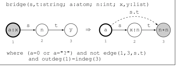
GP’s principal programming constructs are conditional rule schemata. These extend the rules ofSubsection 2.1with expressions in labels and with application conditions. For example, Fig-ure 1shows the declaration of a conditional rule schemabridge, where roots are depicted as nodes with bold borders. Only the left- and right-hand side of the rule schema are declared. By convention, the interface is the unlabelled and rootless graph consisting of the numbered nodes.
bridge(s,t:string; a:atom; n:int; x,y:list)
a:x
1
n
2
s
y
3
t
⇒ a
1
x:n
2
s
n*n
3
t s.t
where (a=0 or a="?") and not edge(1,3,s.t) and outdeg(1)=indeg(3)
Figure 1: Declaration of a conditional rule schema
in the condition must also occur in the left-hand side because their values at execution time are determined by matching the left-hand side with a subgraph of the host graph.
Each variable is declared with a type which is eitherint,string, atomorlist. Types form a subtype hierarchy in which integers and character strings are basic types, both of which are atoms, which in turn are considered as lists of length one. In general, a label in GP is a list of atoms each of which is either an integer or a character string. Labels in host graphs do not contain expressions; they are fixed values in(Z∪Char∗)∗, where Char is the set of available characters.
Lists are constructed by the colon operator which represents list concatenation. For example, the label of node 1 on the left ofFigure 1stands for a list whose first elementais an integer or a character string, followed by a (possibly empty) rest listx. String concatenation is signified by the dot operator, as in the edge labels.t on the right ofFigure 1. Labels in the right-hand side of a rule schema may contain arithmetic expressions such asn∗nin node 3 on the right of
Figure 1.
Besides having labels, both nodes and edges can bemarked. Graphically, a marked node is shaded, and a marked edge is dashed. Marked items in rule schemata can only match marked items in host graphs. Vice versa, marked items in host graphs can only be matched by marked items in rule schemata. Marks are used as boolean flags and should not be confused with roots.
Rule schemata have an optional condition, declared with the keywordwhere. The condition is a boolean expression containing built-in predicates and functions, label expressions, and node identifiers. For example, the subexpressionnot edge(1,3,s.t)inFigure 1demands that there must not be an edge in the host graph from node 1 to node 3 that is labelled with the string s.t(wheresandtstand for the host graph labels of the edges in the left-hand side). To apply the rule schema according to a match of the left-hand side, the condition must evaluate to true for that match and its induced assignment of values to variables.
3.2 Programs
GP programs consist of a finite number of rule schemata and a command sequence which controls their application to a host graph (see Figure 3 for an example program). The main control constructs are: application of a set of conditional rule schemata{r1, . . . ,rn}, where one of the applicable schemata in the set is nondeterministically chosen or otherwise the command fails; sequential compositionP;Qof programsPandQ; as-long-as-possible iterationP! of a program P; and conditional branching statementsifCthenPelseQandtryCthenPelseQ, where C,PandQare arbitrary command sequences.
To execute ifC then P else Q on a stateG (the current graph), first the conditionC is executed onG. If this produces a graph, then this result is disposed andPis executed on state G. Alternatively, ifCfails onG, thenQis executed on G. This behaviour makes it possible to encode complex tests in the conditionCwhich do not alter the current state.
The commandtryCthenPelseQalso first executesConGand, if this fails, executesQ onG. However, ifCproduces a graphH, thenPis executed onHrather than onG.
4
A Matching Algorithm for Rooted Rule Schemata
We present a matching algorithm for rooted rule schemata which extends the corresponding algo-rithms in [4,2]. The main difference is that instead of matching plain graph transformation rules, we have to deal with the syntax of GP 2-rule schemata. In particular, the algorithm must com-pare label expressions of the left-hand side with values in host graph labels and, besides finding matches of the graph structure, compute assignments of values to variables. These assignments are used both in evaluating the application condition of the rule schema and in calculating the labels of new and relabelled items when the rule schema is applied. Another extension to the previous algorithms is that we allow multiple roots in rule schemata and host graphs, while the cited papers assume a single root. Moreover, it is now possible to designate arbitrary nodes as roots whereas before a root had to be identified by a uniquely occurring label.
First we introduce some notation used in the algorithm. Apartial premorphism g: G→H is a pair of partial functionsgV:VG→VH andgE:EG→EH such that for each edgeeinG, if gE(e)is defined thengV(sG(e))andgV(tG(e))are also defined and satisfysH(gE(e)) =gV(sG(e)) andtH(gE(e)) =gV(tG(e)). We write Dom(gV)and Dom(gE) for the sets of nodes and edges on which g is defined. Given partial premorphisms f,g: G→H, f extends g by a node v if Dom(fV) =Dom(gV)∪ {v} and Dom(fE) =Dom(gE). Also, f extends g by an edge e if Dom(fE) =Dom(gE)∪ {e} and Dom(fV) =Dom(gV)∪ {sG(e),tG(e)}. Given a rooted graph
hL,PLiandp∈PL, anedge enumerationforpis a list of edgese1, . . . ,ensuch that{e1, . . . ,en}is the set of all edges reachable fromp,e1is incident top, and fori=2, . . . ,n,eiis incident to the source or target of some edge in{e1, . . . ,ei−1}.
Algorithm Rooted Graph Matching
A← {hh:L−−→par G,/0i |Dom(h) =/0}
whilethere exists an untagged rootp∈PLdo A0← {hh:L
par
−−→G,αh0i |his injective and root-preserving, and
there existshh0,αh0iinAsuch thathextendsh0by p}
tag p
AssignmentUpdate(A0)
fori=1 tondo
Ai← {hh:L par
−−→G,αh0i |his injective and root-preserving, and
there existshh0,αh0iinAi−1such thathextendsh0byei}
ifs(ei)∈PLthentags(ei) ift(ei)∈PLthentagt(ei) AssignmentUpdate(Ai) end for
A←Apn
end while returnA
Figure 2: Algorithm Rooted Graph Matching
matches ofhL,PLiinhG,PGi. The algorithm assumes that each node inLis reachable from some root. It incrementally constructs a setAof pairs of partial premorphismsh:L−−→par Gand partial assignmentsαh. By a partial assignment we mean a partial function Var(L)→(Z∪Char∗)∗, where Var(L)is the set of variables occurring inL. The roots inLare tagged whenever they are matched; initially they are all untagged.
The algorithm calls the procedure AssignmentUpdate, which exploits that expressions in the left-hand side of a GP rule schema are constrained to prevent ambiguous variable assignments. Expressions must not contain arithmetic operators, more than one occurrence of a list variable, or more than one occurrence of a string variable in a single string expression.
Lists and strings are stored internally as doubly-linked lists with pointersfirstandlastpointing to the first and last element. Hence the first and last element of a list or string, as well as the predecessor and successor of the current element, can be accessed in unit time. With this data structure, only the pointersfirstandlastare needed when assigning a value to a list, atom or string variable, as the rest of the list or string can be accessed through thenextandprevoperators.
AssignmentUpdate is omitted for lack of space; we give a brief outline of its operation. The procedure iterates over its input, a set of pairs of partial premorphisms and partial assignments. For each pair hh,αi, it iterates over all untested labels l in the domain ofh. Eachl and cor-responding host graph valueh(l)are evaluated by a local procedure which will also update the partial assignment iflcontains a variable and the two expressions can be matched. In particular, expressions containing a list variable or a string variable are tested by comparing the individual components (atoms or characters) that occur before and after the single variable. If all compo-nents match, then the variable has a unique mapping. This mapping is specified by assigning locations to the first andlast pointers of the string or list variable. This is sufficient; the rest of the string or list can be accessed through the list operators as the value is stored as a doubly linked list in the graph data structure.
Proposition 1(Correctness of Rooted Graph Matching) The algorithm Rooted Graph Match-ing returns the set of all pairshg,αiwhere g:L→G is an injective root-preserving premorphism
andα: Var(L)→(Z∪Char∗)∗is a total assignment such that g:Lα→G is label-preserving.
HereLα is the graph obtained fromLby replacing each variablexwith the value
α(x).
Ac-cording to the semantics of GP 2 [10],gmust be label-preserving after this replacement, that is, it must be a graph morphismLα→G. We omit the proof ofProposition 1for lack of space.
5
Complexity of Rooted Rule Schemata
In this section, we analyse the complexity of the rooted graph matching algorithm and of apply-ing a conditional rule schema with a given match. We make the followapply-ing general assumption.
Assumption 1(Complexity model)
When analysing the complexity of rule schemata and programs, we assume that
1. rule schemata and programs are fixed, and
The first assumption is customary in algorithm analysis where programs are fixed and running time is measured in terms of input size. In our setting, programs consist of fixed rule schemata and the input size is the size of a host graph and its labels.1 The second assumption is consistent with the uniform cost criterion for random access machines, the standard complexity model in algorithm analysis [1,11].
Our matching algorithm assumes that each node in a left-hand graph is reachable from some root. This alone does not guarantee that rule schemata can be applied in time independent of the host graph. To achieve this, we need to impose some more restrictions on the form of rooted rule schemata. We will show that, under mild assumptions on host graphs, rule schemata of the following form can be applied in constant time.
Definition 1(Fast rule schema)
A rule schemaL⇒Rwith application conditioncisfastif
1. each node inLis reachable from some root,
2. LandRdo not contain repeated list, string or atom variables, and
3. cdoes neither contain theedgepredicate nor a teste1=e2ore1!=e2where bothe1ande2 contain a list, string or atom variable.
The first condition ensures that matches can only occur in the neighbourhood of roots. The second condition makes it unnecessary to check the equality of lists or strings, or to copy lists or strings. The third condition rules out tests that require more than constant time.
Applying a conditional rule schemaL⇒Rto a host graphGrequires several phases: finding a root-preserving match ofLinGand constructing the induced variable assignment; checking the dangling condition and the application condition; removing items fromL−K; adding items fromR−K; and relabelling nodes. In the following we focus on the complexity of the matching phase because, in the worst case, it is far slower than the other phases.
We give the following lemma without proof due to lack of space.
Lemma 1 Given a fast rule schema L⇒R and a host graph G, the procedure AssignmentUp-date compares each label in L in constant time with the corresponding label in G.
We can now show that fast rule schemata can be matched in constant time, provided that both node degrees and the number of roots in host graphs are bounded. Thedegreeof a nodevis the sum of the number of edges with sourcevand the number of edges with targetv.
Theorem 1 The algorithm Rooted Graph Matching runs in constant time for fast rule schemata if there are upper bounds on the maximal node degree and the number of roots in host graphs.
Proof. Consider a fast rule schemaL⇒Rand a host graphG. Letlbe the number of roots inL. Letbandrbe upper bounds on the maximal node degree and the number of roots in host graphs respectively.
First we count the number of times the set of partial premorphismsL−−→par Gis updated. We assume a data structure where adding either a node, an edge, or a node and an edge to an existing
morphism takes unit time. There are at most l iterations of the while loop and, within each iteration, at mostm=|EL|iterations of the for loop. Note that, by Assumption1, bothlandm are constants.
Consider the execution of the first iteration of the while loop. First, a single root from L is matched with all unmatched roots in G. Since no roots have been matched yet, r partial morphisms are created. Then, in each iteration, either a single edge or an edge and a node is added to the domain of one of more morphisms in the current set. As node degrees inG are bounded byb, no more thanbadditions can take place. This gives a worst-case running time of r+b|A0|+b|A1|+...+b|Am−1|. The setA0 contains at mostr morphisms,A1contains at most brmorphisms, etc. It follows that the running time isr+br+b2r+. . .+bmr=r∑mi=0bi.
Next, the second root of Lis matched. Since one root in G has already been matched, the maximum size of the new morphism set isbmr(r−1). Hence, by the same argument as before, the maximal running time after the second iteration of the while loop is
r m
∑
i=0
bi+r(r−1) 2m
∑
i=m bi.
After thel-th and final iteration of the while loop, the total running time is bounded by
r m
∑
i=0
bi+r(r−1) 2m
∑
i=m
bi+. . .+r(r−1). . .(r−l+1)
lm
∑
i=(l−1)m bi.
The procedure AssignmentUpdate is called after each update of the set of premorphisms. Each execution checks at most two labels for every premorphism in the set since on each update, at most two new items are added to the domain of the premorphism. Thus, byLemma 1, it follows that the total execution time of Rooted Graph Matching is bounded by a constant factor of the above expression.
Given a match of the left-hand side of a fast rule schema, checking the application condition and the dangling condition, and deleting, adding and relabelling items can be done in constant time. Hence we obtain the following corollary ofTheorem 1.
Corollary 1 Fast rule schemata can be applied in constant time if there are upper bounds on the maximal node degree and the number of roots in host graphs.
Proof sketch. Consider again a fast rule schemaL⇒Rwith conditioncand a host graphG. By
Theorem 1, constructing a premorphismg:L→Gand induced variable assignmentα (or
deter-mining there is no such pair) requires only constant time. We need to prove that the remaining phases of rule schema application can be executed in constant time, too.
checks according to (3) can be done in unit time if the data structure for labels records type information suitably.
The dangling condition for an injective premorphismg:L→Gcan be checked by comparing the degree of each node v in L−K with the degree of its image g(v). We assume a graph representation where nodes are stored together with their indegree and outdegree. This operation then takes time of order|VL|, a constant.
Given a match satisfying the dangling condition, removing the items ing(L−K)can be ex-ecuted in time proportional to|L| − |K|. Similarly, the addition of nodes and edges takes time proportional to|R| − |K|.
Finally, relabelling a string or list only requires redirecting the pointers first and last to a particular label in G. For string concatenation, two more pointer redirections are required to combine the two strings. There are at most|VK|relabellings, so the time needed is proportional to|VK|.
The overall time complexity of a fast rule schema is largely determined by the number of roots in both the rule schema and the host graph. This is to be expected since the number of roots available for matching will increase the number of matches. Indeed, if all nodes were roots, then rooted matching would be identical to conventional graph matching. In practice, we aim to limit the number of roots. For example, in our case study in the next section, we use only one root in both rule schemata and host graphs.
6
Case Study: 2-Colouring
Vertex colouring has many applications [11] and is among the most frequently considered graph problems. We focus on 2-colourability: a graph is2-colourable, orbipartite, if we can assign one of two colours to each node such that the source and target of each edge have different colours.
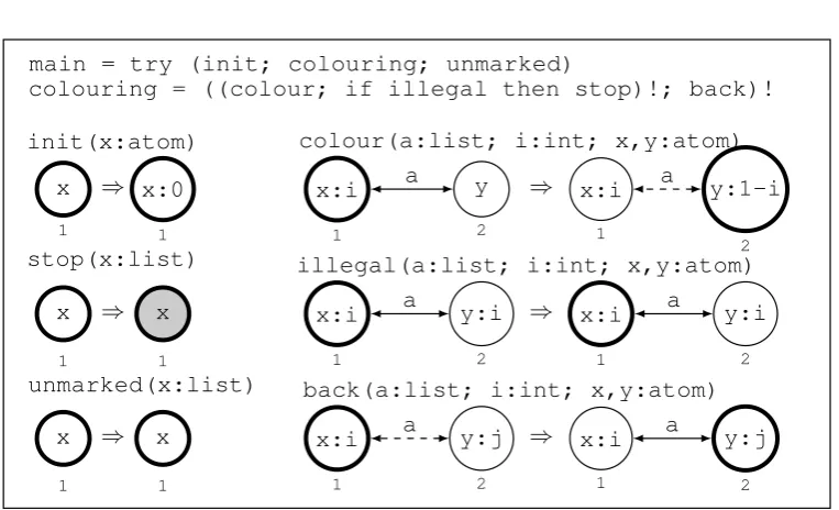
The GP program2colouringinFigure 3expects a connected and unmarked input graph Gwith atomic node labels and a single root. The program will either produce a 2-colouring for Gby appending the integer 0 or 1 to each node label, or returnGunmodified if no 2-colouring exists. For the rest of this section, by arooted graphwe mean a connected graph with a single root.
InFigure 3, the roots in rule schemata are depicted with a thick border. For notational con-venience, the rule schematacolour,illegalandbackcontain bidirectional edges. Each of these rule schemata actually represents a set of two distinct rule schemata with normal edges such that the edge direction is the same in the left- and right-hand side. For example,colour stands for the set{colour1,colour2}wherecolour1 andcolour2differ only by the edge direction. Whencolouris called by the main program,colour1orcolour2is selected non-deterministically and applied. If it is not applicable, then the other rule schema is attempted.
main = try (init; colouring; unmarked)
colouring = ((colour; if illegal then stop)!; back)!
x 1 ⇒ init(x:atom) x:0 1 x 1 ⇒ stop(x:list) x 1 x 1 ⇒ unmarked(x:list) x 1 x:i 1 y 2 a ⇒
colour(a:list; i:int; x,y:atom)
x:i 1 y:1-i 2 a x:i 1 y:i 2 a ⇒
illegal(a:list; i:int; x,y:atom)
x:i 1 y:i 2 a x:i 1 y:j 2 a ⇒
back(a:list; i:int; x,y:atom)
x:i
1
y:j
2
a
Figure 3: GP program2colouring
Upon termination of the macrocolouring, the rule schemaunmarkedchecks whether the root is unmarked or not. If not, then the rule schemaillegalhas detected an edge whose ends have the same colour andstophas marked the root. In this case the input graph is not bipartite and by the semantics of the try command, the input graph is returned as the application of unmarkedfailed. On the other hand, if the root is unmarked, then the whole graph has been correctly coloured.
Proposition 2(Correctness of2colouring) Given a rooted input graph G with atomic node labels, the program2colouringreturns a 2-coloured version of G if G is bipartite, otherwise it returns G unchanged.
We omit the proof for lack of space. Note that each of the nine rule schemata can only be applied at the unique root of the current graph. Therefore the root needs to be moved around, which happens with bothcolourandback. However, care must be taken to prevent the root being moved back and forth between the same nodes forever. The program avoids this kind of looping by marking an edge only when an incident node gets a colour and unmarking this edge whenbackis applied to it (without altering the colours).
We now analyse the time complexity of2colouring. First note that all rule schemata are fast in the sense ofDefinition 1. Hence, byCorollary 1, we know that each rule schema takes only constant time on rooted graphs of bounded degree. Moreover, none of the rule schemata increases any node degree or the number of roots. Hence repeated rule schema applications in program runs preserve the assumptions ofCorollary 1.
copying the input graph and returning the copy in case the command sequence fails.
As to the number of rule schema applications, observe first that the rule schemata init, unmarked,illegalandstopcan be ignored because each of them is applied at most once in a program run. Next, we notice thatcolourreduces the number of uncoloured nodes and backdoes not increase this number. Hencecolouris applied at mostntimes, wherenis the number of nodes in the input graph. Moreover,backcannot be applied more often thancolour because the input graph is unmarked, onlycolourcreates an edge mark, andback removes one edge mark. Thus, there are at most 2napplications ofcolourandback. Altogether, we have shown the following.
Proposition 3(Time complexity of2colouring) On rooted input graphs with atomic node labels and bounded node degree, the running time of 2colouring is linear in the size of graphs.
This is significantly better than what can be achieved with unrooted programs. For, in the worst case of rule schema matching, even a clever algorithm requires at least linear time as it needs to search the complete host graph. Since each node of a bipartite input graph gets coloured, it follows that such a program has at least quadratic running time.
7
Conclusion
We have presented an approach for programming with graph transformation rules in which the bottleneck of graph transformation—the inefficiency of graph matching—is circumvented by using rooted rules which only match in the neighbourhood of host graph roots. Rooted graph transformation has been cleanly embedded in the framework of the double-pushout approach and has been extended to rule schemata in the graph programming language GP.
We have shown an algorithm which matches a large class of rooted conditional rule schemata in constant time, provided that host graphs have bounded node degrees. Our case study demon-strates that algorithms of practical importance, such as graph colouring, can be implemented with rooted GP programs whose time complexity is as good as that of programs in imperative languages. Moreover, we have demonstrated that due to the simplicity of GP and its semantics, the correctness and complexity of rooted graph programs is amenable to formal analysis. Essen-tially, because fast rule schemata can be applied in constant-time, to show that a program with fast rule schemata has a certain time complexityT, it suffices to prove that the maximal number of rule schema applications is of orderT.
In future work, we will consider alternative sufficient conditions that make rooted programs fast. For example, in [4] it is shown that graph transformation rules can be applied in constant time if the outdegree of nodes in host graphs is bounded and the left-hand sides of rules contain a directed path from the root to each node. A corresponding result should hold for fast rule schemata if each node in a left-hand side is reachable from some root by a directed path.
Finally, we will aim at confirming our theoretical results by implementing a rooted version of GP and comparing the performance of graph programs with that of programs in traditional programming languages.
Bibliography
[1] A. V. Aho, J. E. Hopcroft, and J. D. Ullman. The Design and Analysis of Computer Algo-rithms. Addison-Wesley, 1974.
[2] M. Dodds. Graph Transformation and Pointer Structures. PhD thesis, The University of York, 2008.
[3] M. Dodds and D. Plump. Extending C for checking shape safety. InProc. Graph Trans-formation for Verification and Concurrency (GT-VC 2005), volume 154(2) of Electronic Notes in Theoretical Computer Science. Elsevier, 2006.
[4] M. Dodds and D. Plump. Graph transformation in constant time. In Proc. International Conference on Graph Transformation (ICGT 2006), volume 4178 ofLecture Notes in Com-puter Science, pages 367–382. Springer-Verlag, 2006.
[5] H. D¨orr. Efficient Graph Rewriting and its Implementation, volume 922 ofLecture Notes in Computer Science. Springer-Verlag, 1995.
[6] R. Geiß, G. V. Batz, D. Grund, S. Hack, and A. M. Szalkowski. GrGen: A fast SPO-based graph rewriting tool. In Proc. International Conference on Graph Transformation (ICGT 2006), volume 4178 of Lecture Notes in Computer Science, pages 383–397. Springer-Verlag, 2006.
[7] A. Habel and D. Plump. Relabelling in graph transformation. InProc. International Con-ference on Graph Transformation (ICGT 2002), volume 2505 ofLecture Notes in Computer Science, pages 135–147. Springer-Verlag, 2002.
[8] U. Nickel, J. Niere, and A. Z¨undorf. The FUJABA environment. In Proc. International Conference on Software Engineering (ICSE 2000), pages 742–745. ACM Press, 2000.
[9] D. Plump. The graph programming language GP. InProc. International Conference on Algebraic Informatics (CAI 2009), volume 5725 of Lecture Notes in Computer Science, pages 99–122. Springer-Verlag, 2009.
[10] D. Plump. The design of GP 2. In Proc. International Workshop on Reduction Strate-gies in Rewriting and Programming (WRS 2011), volume 82 ofElectronic Proceedings in Theoretical Computer Science, pages 1–16, 2012.
[11] S. S. Skiena.The Algorithm Design Manual. Springer-Verlag, second edition, 2008.