AUSTRALIAN JOURNAL OF BASIC AND
APPLIED SCIENCES
ISSN:1991-8178 EISSN: 2309-8414 Journal home page: www.ajbasweb.com
Open Access Journal
Published BY AENSI Publication
© 2016 AENSI Publisher All rights reserved
This work is licensed under the Creative Commons Attribution International License (CC BY).
http://creativecommons.org/licenses/by/4.0/
To Cite This Article: M. Arumuga Babu, R.Mahalakshmi, S.Kannan, M.Karuppasamypandiyan and A.Bhuvanesh., Economic Dispatch of Distributed Generation Using Backtracking Search Optimization Algorithm. Aust. J. Basic & Appl. Sci., 10(5):127-133, 2016
Economic Dispatch of Distributed Generation Using Backtracking Search
Optimization Algorithm
1M. Arumuga Babu, 2R.Mahalakshmi, 3S.Kannan, 4M.Karuppasamypandiyan and 5A.Bhuvanesh
1Assistant Professor & Head, Dept. of EEE, Tejaa shakthi Institute of Technology for Women, Coimbatore. 2Professor, Dept. of EEE, Kumaraguru of Technology, Coimbatore
3Professor & Head, Dept. of EEE, Ramco Institute of Technology, Rajapalayam 4Assistant Professor, Dept. of EEE, Kalasalingam University, Krishnankoil 5
Research Scholar, Dept. of EEE, Mepco schlenk Engineering College, Sivakasi.
Address For Correspondence:
M. Arumuga Babu, Assistant Professor & Head, Dept. of EEE, Tejaa shakthi Institute of Technology for Women, Coimbatore. E-mail:[email protected]
A R T I C L E I N F O A B S T R A C T
Article history:
Received 12 January 2016 Accepted 22 February 2016 Available online 1 March 2016
Keywords:
Backtracking Search Optimization Algorithm, Differential Evolution, Distributed Generators, Economic Dispatch.
Nowadays, distributed generators (DG) are most widely used in distribution system to satisfy the increasing demand. According to the demand, the dispatch of generator should be modified for economic operation. The economic dispatch (ED) of DGs are normally solved by anyone of the following methods: conventional methods such as Lambda iteration method, Dynamic Programming etc., or optimization technique such as Genetic algorithm (GA), Evolutionary Programming (EP), Differential Evolution (DE) Algorithm etc., These methods of solving ED problem require comparatively large computation time. Therefore, it is important to estimate real power dispatch val-ues within a short period. This paper presents the ED of various DGs for different demands using Backtracking Search Optimization Algorithm (BSA). In this work two diesel engines, single units of wind turbine generator and fuel cell are used as DG. The ED problem is solved for IEEE 33 bus distribution system by BSA and DE. The test result shows that the BSA method is better for ED of DG than DE.
INTRODUCTION
According to the definition of CIGRE (1999), Distributed Generation (DG) is defined as the generating plant with a capacity of less than 100 MW, usually connected to the distribution networks that are neither cen-trally planned nor dispatched. One of the drawbacks of using non-renewable DG in distribution system is its fuel cost. Hence, to reduce this fuel cost the DGs should be optimally dispatched.
Economic dispatch (ED) is one of the most important optimization problems in power system operation and planning. It is to economically dispatch the generators according to demand while satisfying the physical and operational constraints. Classical methods such as Lambda iteration, Base point Participation factor, Gradient method, Newton’s method and Lagrange multiplier method can solve ED problem under the assumption that the incremental cost curves of the generating units are monotonically increasing piecewise-linear functions. How-ever, in reality, the cost curves of generating units are non-convex. Classical based techniques fail to address these types of problems satisfactorily and lead to sub optimal solutions producing huge revenue loss over time. According to Basu and Chowdhury (2013), Dynamic programming (DP) can solve ED problem with inherently nonlinear and discontinuous cost curves. But it suffers from the curse of dimensionality or local optimality.
optimization (BBO) by Bhattacharya A and Chattopadhyay PK (2010), Simulated Annealing (SA) by Wong KP, Fung CC (1993) etc., The main drawbacks of these optimization algorithms are time consuming because for every demand the programs needs to be run to get optimal result. An On-line ED of various non-renewable DGs for various demands using Artificial Neural Networks namely Back Propagation Neural Network (BPNN) and Radial Basis Function Neural Network (RBFNN) are presented by Arumuga Babu et al. (2014). BSA for nu-merical optimization problems have been implemented by Pinar Civicioglu (2013). This paper presents ED of four DGs using BSA.
Problem Formulation:
In this section, the objective function for the fuel cost and pollutant emission minimization by Wanxing Sheng et al. (2013) is explained in detail.
2.1.Fuel Cost and Pollutant Emission Minimization:
The objective is to minimize the fuel cost and the pollutant emission penalty, which reflects the impact of energy utilization on the environment. It can be expressed as follows:
(1)
where is the energy consumption cost and is the pollutant emission penalty. The fuel cost normally can be further expressed as follows:
(2)
where , , and are the quadratic cost coefficients of the -th DG, and DG is the number of distributed
generators (DG). DG is the real power output of the -th generator.
DG is the vector of real power outputs of generators and defined as follows:
(3)
The pollutant emission quantity can be obtained based on DG output. Then, based on the penalty standard, the environmental penalty for pollutant emission is calculated as follows:
(4)
where is pollutant ’s emission quantity and is the penalty standard of pollutant .
Modelling Of Distributed Generation:
In this section, the Diesel generator, wind turbine generator and fuel cell plant are explained in detail [2].
2.2.Diesel generator:
The objective function in a diesel generator consists of the fuel cost function similar to the conventional cost functions used for the fossil-fuel generating plants.
(5)
where
FDiesel is the diesel generation cost;
PDiesel,it is the diesel generation output in kW of unit i at time t;
αdi, βdi, γdi are the coefficients of i-th generator fuel cost; Nd is the number of diesel generator;
t and T are the time index and scheduling period.
2.3.Wind-turbine generator:
The wind-turbine generator is modelled by the characteristics of variable output because the generation in a wind-turbine generator is determined by the strength of the wind.
(6)
(7)
(8)
(9)
(10)
where Vit, Vcutin,i, Vcutout,i and Vrated,i are the t-th time wind velocity, cut-in velocity, cut-out velocity and rated
velocity in m/sec of unit i respectively;
Pwind,it and Pwind,rated,i are the wind power generation of unit i at time t and rated wind power output of unit i
respectively;
βwi maintenance and operating cost in $/kW; Nw is the number of wind-turbine generators; Fwind is the wind generation cost.
2.4.Fuel-cell plant:
The operating cost in fuel-cell system takes the fuel costs and includes the efficiency for fuel to generate electric power. When fuel is transformed into power, the cost function considers the efficiency of fuel cell. Fuel-cell is the most efficient system among all fossil-fuel energy sources.
(12)
where FFC is the fuel-cell generation cost;
βnatural is the natural gas cost in $/kg;
PFC, it is the fuel-cell generation of i-th unit at time t;
ηFC,i is the fuel-cell efficiency of unit i; NFC is the number of fuel-cell plants.
Review And Implementation Of Bsa For Ed Problem:
The basic operating principle of BSA and implementation of BSA for ED problem are explained in this section. BSA is a population-based iterative EA designed to be a global minimizer. BSA can be explained by dividing its functions into five processes as is done in other EAs: initialization, selection-I, mutation, crossover and selection-II [11].
2.5.Initialization:
BSA initializes the population P with Eq. (13):
~ U(lowj , upj) (13)
for i = 1,2,3,...,N and j = 1,2,3,...,D, where N and D are the population size and the problem dimension, re-spectively, U is the uniform distribution and each Pi is a target individual in the population P.
2.6.Selection-I:
BSA’s Selection-I stage defines the historical population oldP to be used for calculating the search direc-tion. The initial historical population is determined using Eq. (14):
oldPi,j~ U(lowj, upj) (14)
BSA has the option of redefining oldP at the beginning of each iteration through the ‘if-then’ rule in Eq. (15):
if a<b then oldP := P|a,b ~ U(0,1), (15)
where :=is the update operation. Eq. (15) confirms that BSA designates a population belonging to a ran-domly selected previous generation as the historical population and remembers this historical population until it is changed. Thus, BSA has a memory. After oldP is determined, Eq. (16) is used to randomly change the order of the individuals in oldP:
oldP := permuting (oldP). (16)
The permuting function used in Eq. (16) is a random shuffling function.
2.7.Mutation:
BSA’s mutation process generates the initial form of the trial population Mutant using Eq. (17).
Mutant = P+F. (oldP-P). (17)
In Eq. (17), F controls the amplitude of the search-direction matrix (oldP-P). Because the historical popula-tion is used in the calculapopula-tion of the search-direcpopula-tion matrix, BSA generates a trial populapopula-tion, taking partial advantage of its experiences from previous generations. This paper uses the value F=3.rndn, where rndn~ N(0,1) (N is the standard normal distribution).
BSA’s crossover process generates the final form of the trial population T. The initial value of the trial population is Mutant, as set in the mutation process. Trial individuals with better fitness values for the optimiza-tion problem are used to evolve the target populaoptimiza-tion individuals. BSA’s crossover process has two steps. The first step calculates a binary integer-valued matrix (map) of size N. D that indicates the individuals of T to be manipulated by using the relevant individuals of P. If mapn,m=1, where n ε {1; 2; 3;...; N}and m ε{1; 2; 3;...; D},
T is updated with Tn;m:=Pn;m.
2.9.Selection-II:
In BSA’s Selection-II stage, the Tis that have better fitness values than the corresponding Pis are used to
update the Pis based on a greedy selection. If the best individual of P (Pbest) has a better fitness value than the
global minimum value obtained so far by BSA, the global minimizer is updated to be Pbest, and the global
mini-mum value is updated to be the fitness value of Pbest.
2.10.Implementation of BSA to Optimal DG Dispatch Problem:
The BSA approaches for solving the fuel cost and pollutant emission minimization for distribution system are as follows:
i. Read bus data, line data.
ii. Read data for BSA operations i.e. maximum iteration limit, number of population, the decision vari-able, lower and upper limit of decision varivari-able, scaling factor F.
iii. Initialize old population Pold.
iv. Generate population randomly, where decision variable is within its feasible bound. v. Perform mutation and crossover.
vi. In Selection-II, if Tis have better fitness values than Pis, update the Pis based on a greedy selection.
vii. If Pbest has a better fitness value than the global minimum value obtained, the global minimum value is
updated to be the fitness value of Pbest.
viii. Using selected best vector value run the objective to find minimum fuel cost and pollutant emission cost.
ix. Best value selected will be the next parent for the next Population. x. Increase the generation gen = gen+1.
xi. Print the corresponding selected best valuefor the fuel cost and pollutant emission minimization. xii. Stop the program.
RESULTS AND DISCUSSION
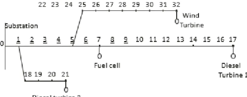
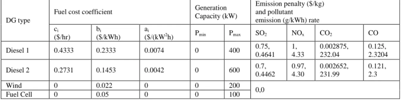
The proposed BSA has been applied to IEEE 33 bus distribution system to minimize the fuel cost and the pollutant emission penalty cost and shown in Figure 1. The study is carried out for 24 hours. The demand is assumed to be for every one hour. There are totally four types of DGs are considered having two diesel genera-tors, one wind generator and one fuel cell. The assumed load demand for a day is shown in Figure 2. The wind speed for a whole day is shown in Figure 3. The fuel cost coefficient, generation capacity, emission penalty and pollutant emission rate for diesel, wind and fuel cell is presented in Table 1. The efficiency of fuel cell is 90%. The cut-in and cut-out velocity of wind is 5 and 15 m/sec respectively. The rated wind velocity is 10 m/sec. The simulation studies were carried out using MATLAB.
Fig. 2: Demand for 24 hours
Fig. 3: Wind Speed for 24 hours
Table I: Generation Capacity, Fuel cost coefficient, emission penalty and pollutant emission rate for different DG
DG type
Fuel cost coefficient Generation
Capacity (kW)
Emission penalty ($/kg) and pollutant
emission (g/kWh) rate ci
($/hr) bi ($/kWh)
ai
($/(kW2h) Pmin Pmax SO2 NOx CO2 CO
Diesel 1 0.4333 0.2333 0.0074 0 400 0.75,
0.4641 1, 4.33 0.002875, 232.04 0.125, 2.3204
Diesel 2 0.2731 0.1453 0.0042 0 600 0.7,
0.4462 0.97, 4.30 0.002652, 231.99 0.121, 2.3
Wind 0 0.022 0 0 200
0,0
Fuel Cell 0 0.05 0 0 100
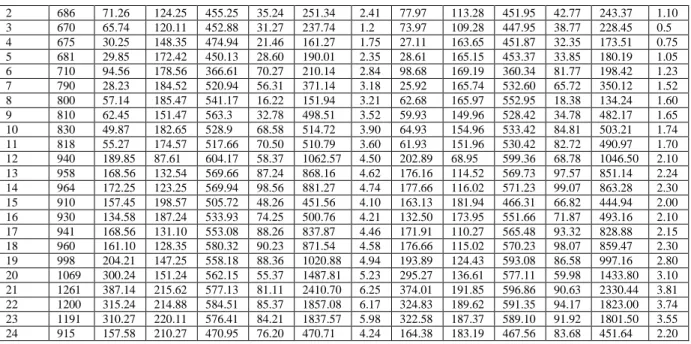
This system consists of 33 bus and 32 branches with a total real power load of 3,715 kW. The base case to-tal system real power loss is 211.23 kW. Four DGs namely Diesel generator 1, Diesel Generator 2, Wind Gen-erator and Fuel cell are placed in bus 17, 21, 32, and 7 respectively. The main grid supplies 3,715 kW to meet the base load demand. The additional demand is met by DG. The real power schedule for 24 hours with mini-mum fuel/pollution emission penalty cost obtained using BSA and DEA are given in Table 2.
Table 2The real power schedule with minimum fuel/pollution emission penalty cost
Hours De-mand (kW)
DEA BSA
2 686 71.26 124.25 455.25 35.24 251.34 2.41 77.97 113.28 451.95 42.77 243.37 1.10 3 670 65.74 120.11 452.88 31.27 237.74 1.2 73.97 109.28 447.95 38.77 228.45 0.5 4 675 30.25 148.35 474.94 21.46 161.27 1.75 27.11 163.65 451.87 32.35 173.51 0.75 5 681 29.85 172.42 450.13 28.60 190.01 2.35 28.61 165.15 453.37 33.85 180.19 1.05 6 710 94.56 178.56 366.61 70.27 210.14 2.84 98.68 169.19 360.34 81.77 198.42 1.23 7 790 28.23 184.52 520.94 56.31 371.14 3.18 25.92 165.74 532.60 65.72 350.12 1.52 8 800 57.14 185.47 541.17 16.22 151.94 3.21 62.68 165.97 552.95 18.38 134.24 1.60 9 810 62.45 151.47 563.3 32.78 498.51 3.52 59.93 149.96 528.42 34.78 482.17 1.65 10 830 49.87 182.65 528.9 68.58 514.72 3.90 64.93 154.96 533.42 84.81 503.21 1.74 11 818 55.27 174.57 517.66 70.50 510.79 3.60 61.93 151.96 530.42 82.72 490.97 1.70 12 940 189.85 87.61 604.17 58.37 1062.57 4.50 202.89 68.95 599.36 68.78 1046.50 2.10 13 958 168.56 132.54 569.66 87.24 868.16 4.62 176.16 114.52 569.73 97.57 851.14 2.24 14 964 172.25 123.25 569.94 98.56 881.27 4.74 177.66 116.02 571.23 99.07 863.28 2.30 15 910 157.45 198.57 505.72 48.26 451.56 4.10 163.13 181.94 466.31 66.82 444.94 2.00 16 930 134.58 187.24 533.93 74.25 500.76 4.21 132.50 173.95 551.66 71.87 493.16 2.10 17 941 168.56 131.10 553.08 88.26 837.87 4.46 171.91 110.27 565.48 93.32 828.88 2.15 18 960 161.10 128.35 580.32 90.23 871.54 4.58 176.66 115.02 570.23 98.07 859.47 2.30 19 998 204.21 147.25 558.18 88.36 1020.88 4.94 193.89 124.43 593.08 86.58 997.16 2.80 20 1069 300.24 151.24 562.15 55.37 1487.81 5.23 295.27 136.61 577.11 59.98 1433.80 3.10 21 1261 387.14 215.62 577.13 81.11 2410.70 6.25 374.01 191.85 596.86 90.63 2330.44 3.81 22 1200 315.24 214.88 584.51 85.37 1857.08 6.17 324.83 189.62 591.35 94.17 1823.00 3.74 23 1191 310.27 220.11 576.41 84.21 1837.57 5.98 322.58 187.37 589.10 91.92 1801.50 3.55 24 915 157.58 210.27 470.95 76.20 470.71 4.24 164.38 183.19 467.56 83.68 451.64 2.20
The result show that the BSA performs better than DEA with its quicker execution time and lesser penalty cost. The comparison of Fuel/ Emission penalty cost obtained by BSA and DEA is shown in Figure 4.
Fig. 4: Comparison of Fuel/ Emission penalty cost obtained by BSA and DEA
The main objective is to reduce the Fuel/ Emission penalty cost. BSA integrates Wind turbine generator in more amount depends on its availability. So the Fuel/ Emission penalty cost in BSA is lesser DEA. The ED of DG by BSA for 24 hours is shown in Figure 5.
Conclusion:
Nowadays power crisis is one of the main concerns in the developing countries all over the world. The pro-duction is not sufficient to meet the demands of consumers. So DGs are most widely installed in distribution system to satisfy the increasing demand. Under these condition, the power system should be efficient in ED, which reduces the total generating cost.
This paper has proposed BSA based ED that considers wind power penetration. Simulation studies have been conducted on an IEEE 33-bus system with the objective of minimizing the Fuel/ Emission penalty cost with the wind power penetration of the power system. The results indicate that BSA provides a more reliable solution set for power system dispatch than DE due to its excellent convergence performance.
REFERENCES
CIGRE., 1999. Impact of increasing contribution of dispersed generation on the power system. Working Group, 37(23).
Basu, M. and A. Chowdhury, 2013. Cuckoo search algorithm for economic dispatch. Energy, 60: 99-108. Walter, D.C and G.B. Sheble, 1993. Genetic algorithm solution of economic dispatch with Valve point loading. IEEE Transactions on Power Systems, 8: 1325-32.
Cheng, P.H and H.C. Chang, 1995. Large scale economic dispatch by genetic algorithm. IEEE Transactions on Power Systems, 10(4): 1919-26.
Yang, H.T., P.C. Yang and C.L. Huang, 1996. Evolutionary programming based economic dispatch for units with non-smooth fuel cost functions, IEEE Transactions on Power Systems, 11: 112-18.
Gaing, Z-L., 2003. Particle swarm optimization to solving the economic dispatch considering the generator constraints. IEEE Transactions on Power Systems, 18(3): 1187-95.
Panigrahi, B.K., S.R. Yadav, S. Agrawal and M.K. Tiwari, 2007. A clonal algorithm to solve economic load dispatch. Electric Power Systems Research, 77(10): 1381-89.
Wang, S.K., J.P. Chiou and C.W. Liu, 2007. Non-smooth/non-convex economic dispatch by a novel hybrid differential evolution algorithm. IET Generation, Transmission and Distribution, 1(5): 793-803.
Bhattacharya A and P.K. Chattopadhyay, 2010. Biogeography-based optimization for different economic load dispatch problems. IEEE Transactions on Power Systems, 25(2): 1064-77.
Wong, K.P and C.C. Fung, 1993. Simulated annealing based economic dispatch algorithm. IEEE Proceed-ings Generation Transmission and Distribution, 140(6): 509-15.
Arumuga Babu, M., R. Mahalakshmi, S. Kannan, M. Karuppasamypandiyan and A. Bhuvanesh, 2014. On-line Economic Dispatch of Distributed Generation Using Artificial Neural Networks. In: 5th International Con-ference on Swarm, Evolutionary, and Memetic Computing, pp: 275-283.
Pinar Civicioglu, 2013. Backtracking Search Optimization Algorithm for numerical optimization problems. Applied Mathematics and Computation, 219: 8121–8144.