COMPARISON OF VARIABLE SELECTION METHODS
Elizabeth Koehler Rowley
A dissertation submitted to the faculty of the University of North Carolina at Chapel Hill in partial fulfillment of the requirements for the degree of Doctor of Public Health in the
Department of Biostatistics in the Gillings School of Global Public Health.
Chapel Hill 2019
Approved by:
c
2019
ABSTRACT
Elizabeth Koehler Rowley: Comparison of Variable Selection Methods (Under the direction of Annie Green Howard and Chirayath Suchindran)
Use of classic variable selection methods in public health research is quite common. Many criteria, and various strategies for applying them, now exist including forward selection, backward elimination, stepwise selection, best-subset selection and so on, but all suffer from similar drawbacks. Chief among them is a failure to account for the uncertainty contained in the model selection process. Ignoring model uncertainty can cause several serious problems. Variance estimates are generally underestimated, p-values are generally inflated, prediction ability is overestimated, and results are not reproducible in another dataset.
Modern variable selection methods have become increasingly popular, especially in applications of high-dimensional or sparse data. Some of these methods were developed to address the short-comings of classic variable selection methods, such as backward elimination and stepwise selection methods. However, it remains unclear how modern variable selection methods behave in a classical, meaning non-high-dimensional, setting.
A simulation study investigates the estimation, predictive performance and variable selec-tion capabilities of three representative modern variable selecselec-tion methods: Bayesian model averaging (BMA), stochastic search variable selection (SSVS), and the adaptive lasso. These three methods are considered in the setting of linear regression with a single variable of interest which is always included in the model.
ACKNOWLEDGMENTS
Thank you to my wonderful family, your love and support have carried me to this finish line. Saying yes to you, Neil Rowley, is far and away the smartest thing I have ever done. Your inspiring determination, patience, gentle encouragement, and unfailing love are essential to me in this, and every, endeavor. My sweet Helen, you have made this the most joyful dissertation experience a mother could imagine. My parents, Mary and Tom Koehler, your example always emboldened me to try my very best and have faith that God will take care of the rest. Thank you for endlessly listening to all my rambles, giving excellent advice, and for providing a concrete example of unconditional love. Thank you to the best siblings, Joey, Christine, and Margaret whose loving support is so appreciated.
I would like to thank Dr. Annie Green Howard and Dr. Chirayath Suchindran for their expertise and enthusiasm while completing this project. This dissertation had many twists and turns and I am grateful that you were both eager to encourage me to the finish. I would also like to thank Dr. Matt Psioda. His generous contribution of ideas and time have been invaluable to this work. I have benefited greatly by getting to observe Dr. Amy Herring and Dr. Penny Gordon-Larsen in action. Their example of women passionately using their abilities to improve public health has been inspiring.
I am particularly indebted to my friends who have brightened my entire experience at UNC. Far from being competitors, you were always quick to smile, eager to offer any assistance, and genuine in concern. This dissertation would, quite frankly, not have even been attempted without your friendship. I am very grateful for each of you!
TABLE OF CONTENTS
LIST OF TABLES . . . xi
LIST OF FIGURES . . . xii
CHAPTER 1: INTRODUCTION . . . 1
1.1 Motivation . . . 1
1.2 Some Modeling Challenges in the China Health and Nutrition Survey . . . 3
1.2.1 About CHNS . . . 3
1.2.2 Predicting Visceral Adipose Tissue . . . 4
1.3 Notation . . . 5
1.3.1 Linear Model Review . . . 5
CHAPTER 2: LITERATURE REVIEW . . . 7
2.1 Defining Modeling Error . . . 7
2.2 Sequential Testing Techniques: Forward, Backward, and Stepwise . . . 9
2.2.1 Variable Selection Criteria Used in Comparing Models . . . 10
2.2.2 Backward Elimination . . . 12
2.2.3 Forward Selection . . . 12
2.2.4 Two-Stage Selection . . . 13
2.3 Change in Effect, CIE . . . 13
2.5 Stochastic Search Variable Selection (SSVS) . . . 16
2.6 Adaptive Lasso . . . 18
2.7 Previous Work Comparing Variable Selection Criteria and Methods . . . 19
2.7.1 Popularity of Variable Selection Methods . . . 19
2.7.2 Debates about Best Criterion in Sequential Analysis . . . 20
2.7.3 Model Uncertainty . . . 23
2.7.4 Previous Variable Selection Comparisons . . . 24
2.8 Summary . . . 26
CHAPTER 3: APPLYING MODERN VARIABLE SELECTION TECHNIQUES TO A CLASSIC LINEAR REGRESSION SETTING . . . 27
3.1 Introduction . . . 27
3.2 Background and Review of Representative Modern Variable Selection Methods . . . 31
3.2.1 Bayesian Model Averaging . . . 31
3.2.2 Stochastic Search Variable Selection (SSVS) . . . 33
3.2.3 Adaptive Lasso . . . 35
3.2.4 Classical Variable Selection Methods . . . 36
3.3 Motivating Example . . . 36
3.4 Design of the Simulation Study . . . 37
3.4.1 Data Generation . . . 38
3.4.2 Variable Selection . . . 40
3.4.3 Quantities of Interest . . . 42
3.5 Simulation Results . . . 44
3.5.1 Model Probabilities . . . 44
3.5.3 Estimation of the Main Effect . . . 48
3.5.4 Predictive Performance . . . 52
3.5.5 Agreement . . . 55
3.6 Summary and Limitations . . . 56
3.7 Discussion . . . 57
CHAPTER 4: A COMPARISON OF TRADITIONAL VARIABLE SELECTION METHODS WITH BAYESIAN MODEL AVERAGING IN LOGISTIC REGRESSION MODELS . . . 62
4.1 Introduction . . . 62
4.2 Background and Review of Commonly Used Variable Selection Methods . . . 65
4.2.1 Sequential Testing Techniques: Forward, Backward, and Stepwise . . . 66
4.2.2 Change-in-Effect Methods, CIE . . . 67
4.2.3 Bayesian Model Averaging . . . 68
4.3 Motivating Example . . . 70
4.4 Design of the Simulation Study . . . 71
4.4.1 Data Generation . . . 71
4.4.2 Variable Selection . . . 74
4.4.3 Quantities of Interest . . . 76
4.5 Simulation Results . . . 78
4.5.1 Model Probabilities . . . 78
4.5.2 Variable Probabilities . . . 80
4.5.3 Estimation of the Main Effect . . . 83
4.5.4 Predictive Performance . . . 86
4.6 Summary and Limitations . . . 91
4.7 Discussion . . . 94
CHAPTER 5: PREDICTING VISCERAL ADIPOSE TISSUE WITH BAYESIAN MODEL AVERAGING IN THE CHINA HEALTH AND NUTRITION SURVEY . . . 98
5.1 Introduction . . . 98
5.2 Methods . . . 100
5.2.1 The China Health and Nutrition Survey . . . 100
5.2.2 Visceral Adipose Tissue . . . 100
5.2.3 Anthropometry . . . 101
5.2.4 Demographic Variables . . . 101
5.2.5 Statistical Analyses . . . 101
5.3 Results . . . 102
5.3.1 Participant Characteristics . . . 102
5.3.2 Prediction of VF with Anthropometrics . . . 105
5.4 Discussion . . . 108
CHAPTER 6: CONCLUSION . . . 111
APPENDIX A: SUPPLEMENTAL MATERIALS FOR CHAPTER 3 . . . 113
APPENDIX B: SUPPLEMENTAL MATERIALS FOR CHAPTER 4 . . . 116
APPENDIX C: SUPPLEMENTAL MATERIALS FOR CHAPTER 5 . . . 121
LIST OF TABLES
3.1 Explanatory Variable Correlations for Data Generation. . . 39
3.2 Estimation of Variable of Interest: Percent Bias. . . 49
3.3 Estimation of Variable of Interest: Variance and Coverage. . . 52
3.4 Agreement. . . 55
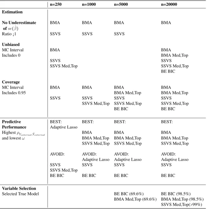
3.5 Summary. . . 61
4.1 Explanatory Variable Correlations for Data Generation. . . 73
4.2 Estimation of Variable of Interest: Percent Bias. . . 84
4.3 Estimation of Variable of Interest: Variance and Coverage. . . 86
4.4 Agreement. . . 88
4.5 Probability that Agreement is on the True Model. . . 88
4.6 Summary. . . 93
5.1 Sample Characteristics by Sex. . . 103
5.2 Anthropometry by Visceral Fat Score. . . 104
5.3 Summary of Top 5 Models . . . 106
5.4 Estimation of Variable of Interest. . . 107
A.1 Simulation Design. . . 113
A.2 Variable Inclusion Probabilitiesn=1000. . . 114
A.3 Variable Inclusion Probabilitiesn=20000. . . 115
B.1 Selection of the True Model . . . 116
B.2 Estimation of Variable of Interest: Percent Bias. . . 117
B.3 Estimation of Variable of Interest: Variance and Coverage. . . 118
LIST OF FIGURES
2.1 Citations of Modern Variable Selection Methods. . . 21
3.1 Citations of Modern Variable Selection Methods. . . 29
3.2 Probability of Selecting the True Model. . . 45
3.3 Variable Inclusion Probabilities. . . 51
3.4 Percent Bias by SE Ratio. . . 54
3.5 Predictive Performance: ρY external,Yˆexternal andω. . . 60
4.1 Probability of Selecting the True Model. . . 79
4.2 Variable Inclusion Probabilities. . . 82
4.3 Percent Bias by SE Ratio. . . 89
4.4 Prediction Capabilities: DY external,P(Yˆ=1)external and over−f it. . . 90
CHAPTER 1: INTRODUCTION
1.1 Motivation
Statistical models are a fundamental tool for the public health researcher. Successful analysis certainly depends on studying the appropriate group of patients, selecting the correct model family, and accurately interpreting the results. However, selecting the variables to include in the model is crucial not only for answering the scientific question, but variable selection is also critical in understanding the replicability of the conclusions. This dissertation explores the effects of modern and classical variable selection techniques relating to three central goals of statistical models: effect estimation, outcome prediction, and understanding variable relationships.
Viallefont et al. 2001, Sun et al. 1996, Hurvich and Tsai 1990).
Model uncertainty can be appropriately represented if estimates from every model consid-ered are somehow accounted for (Buckland et al. 1997). Bayesian model averaging (BMA) provides an opportunity for exploring many possible models while appropriately accounting for the uncertainty surrounding variable selection (Draper 1995, Raftery 1995, Raftery et al. 1997, Hoeting et al. 1999). BMA is only one of several statistical methods developed for
appropriately accounting for model uncertainty but has the advantage of providing the best predictive qualities (George 2000). Stochastic search variable selection (SSVS) is a Bayesian variable selection method initially proposed as a clever way to focus on promising subsets of variables (George and McCulloch 1993). Although both methods have been applied in other fields, methods which account for model uncertainty have yet to see much use in public health (Walter and Tiemeier 2009).
Large population studies typically contain many related variables and selecting between these related variables can be quite challenging. Failure to acknowledge model uncertainty can hinder the public health researcher’s ability to coalesce seemingly disparate results from multiple studies of the same scientific question into knowledge. According to a study by Walter and Tiemeier (2009) of the articles presented inAmerican Journal of Epidemiology, Epidemiology,European Journal of Epidemiology, andInternational Journal of Epidemiology
in 2008, 27.7% of authors used only prior knowledge to build their model, 19.7% used a form of stepwise methods, 14.7% used change in effect methods, and 3% used other methods such as propensity scores or principal components. None of the 300 articles reviewed used ridge regression or shrinkage methods, while a 35% did not disclose their model building strategy, rendering their results uninterpretable. This report suggests methods which directly account for model uncertainty, such as BMA, are either unknown or not easily accessed by those publishing in public health journals.
selection methods both modern (SSVS and adaptive lasso) and classic (backward elimination, two-stage method, and change-in-effect). Variable selection methods are compared on their abilities to estimate a coefficient, to predict an outcome, and to select variables belonging in the true model. These methods are applied to linear and logistic regression in a study where a single variable of interest exists in the presence of several correlated potential covariates. BMA is also used in an applied setting to demonstrate its use and its advantages. In these comparisons and example, this work aims to make BMA better known and more accessible to public health researchers.
1.2 Some Modeling Challenges in the China Health and Nutrition Survey
1.2.1 About CHNS
The China Health and Nutrition Survey (CHNS) collected health data in 361 communities (15 provinces and autonomous cities/districts of Beijing, Chongqing, Guangxi, Guizhou, Hei-longjiang, Henan, Hubei, Hunan, Jiangsu, Liaoning, Shaanxi, Shandong, Shanghai, Yunnan, and Zhejiang) throughout China in ten survey rounds from 1989 to 2015. Using a multistage, random cluster design, a stratified probability sample was used to select counties and cities stratified by income and urbanicity. Communities and households were then randomly selected from these strata. Survey procedures have been described elsewhere (Popkin 2010). The study was approved by the Institutional Review Board at the University of North Carolina at Chapel Hill, the China-Japan Friendship Hospital, the Ministry of Health and China, and the Institute of Nutrition and Food Safety, China Centers for Disease Control. Participants gave informed consent.
suffered from collinearity or over-parameterization.
1.2.2 Predicting Visceral Adipose Tissue
A more specific challenge arises from a particular scientific interest. There is heterogeneity in the metabolic risk of obesity, some obese individuals are at very high metabolic risk, while others are not and being able to predict people who fall in this category is critical for targeting intervention and for understanding the health of a population. While there is debate about which depot of fat may be causally responsible for metabolic complications of obesity (Fabbrini et al. 2009, Klein 2004), visceral fat has been shown to be associated with metabolically abnormal obesity (Pouliot et al. 1992, Banerji et al. 1995, Gastaldelli et al. 2002). Visceral fat has stronger associations with cardio-metabolic diseases than BMI (Wajchenberg 2000, Fontana et al. 2007, Saito et al. 2012, Beaumont et al. 2016), the standard measure of obesity.
Visceral adipose tissue (VAT) can be expensive to measure and may not be historically available in large population studies. Computed tomography (CT) and magnetic resonance imaging (MRI) are considered the gold standard of VAT measurement (Rankinen et al. 1999, Seidell et al. 1990, Koester et al. 1992, Ross et al. 1992, Van der Kooy et al. 1993). Dual-energy x-ray absorptiometry (DXA) whole body scans have been suggested as an alternative (Snijder et al. 2002, Bertin et al. 2000, Direk et al. 2013). None of these measuring techniques are feasible in large population studies. Instead, a variety of anthropometric measures have been suggested as indices of VAT. Waist circumference (Pouliot et al. 1994, Grundy et al. 2013, Ross et al. 1996) and waist-to-hip ratio (Ashwell et al. 1985, Rankinen et al. 1999) have been found to correlate with visceral fat. Body mass index (BMI) is used to define obesity and is commonly used in clinical and epidemiological studies (Smalley et al. 1990, Spiegelman et al. 1992). Other measures considered with varying success in multivariable models have included
circumference (Goel et al. 2008), conicity index (Pinho et al. 2017), sagittal diameter (Pinho et al. 2017), neck circumference (Pinho et al. 2017). Investigating the predictive ability of more readily accessible anthropometric and demographic measures in a multivariable model is an important step in exploiting the richness of existing population studies to better understand the role of visceral fat in the development of metabolically abnormal obesity. Further, a predictive model could help establish better identification of metabolically abnormal obesity in a clinical setting.
1.3 Notation
1.3.1 Linear Model Review
To better understand the competing methods of variable selection, we need to first review linear models. Linear models are devised to investigate the relationship between the response, Yiand the explanatory variablesxi0, . . . , xip. Assume there arensubjects,i=1. . . , n, withp variables recording their traits. A linear model is of the form
Yi =β0+β1φ1(Xi1) +. . .+βpφp(Xip) +i (1.1)
i ∼N(0, σ2) (1.2)
Note,φ1, . . . φM, can be nonlinear functions. The predicted values ofY are denoted and are defined as
ˆ
whereβˆj are the estimates which minimize the squared error, also called the residual sum of squares, RSS.
RSS= n ∑ i=1
(Yi−βˆ0−βˆ1φ1(Xi1) −. . .−βˆpφp(Xip))2 (1.4)
For convenience, we will use matrix notation as shown below.
Y= (Y1, . . . , Yn)′ (1.5)
Xi= (Xi1, . . . , Xip) (1.6)
X= (X1, . . . , Xn)′ (1.7)
β= (β0, . . . , βm)′ (1.8)
Y n×1=
X n×p
β p×1
+ ε n×1
(1.9)
Continuing with the matrix notation, the estimates ofβ, predicted values and RSS are shown.
ˆ β= (X′
X)−1 X′
Y (1.10)
ˆ
Y=X ˆβ (1.11)
RSS = ∥Y−Yˆ∥2 (1.12)
CHAPTER 2: LITERATURE REVIEW
It is helpful to review types of modeling error. We the describe the various variable selection strategies used in this dissertation. Lastly, we examine existing comparisons and critiques of these methods.
2.1 Defining Modeling Error
In order to be able to determine an appropriate parsimonious model, it is useful to consider ways to quantify model error beyond the RSS. Here we define modeling error, ME, and prediction error, PE. Consider two independent samples drawn from a single population, sample A and sample B. Suppose we use sample A to build a model and sample B to examine the model’s prediction ability (Seber and Lee (2003)).
YA′= (YA1, . . . , YAn) (2.1) YB′= (YB1, . . . , YBm) (2.2)
Again,Y represents the response and we assumeYA andYB have covariance matrices of σ2I
nand σ2Im respectively. LetXrepresent the covariates withXai′ andX ′
XA= ⎡⎢ ⎢⎢ ⎢⎢ ⎢⎢ ⎢⎢ ⎣
X′ a1 ⋮
X′ an
⎤⎥ ⎥⎥ ⎥⎥ ⎥⎥ ⎥⎥ ⎦
XB = ⎡⎢ ⎢⎢ ⎢⎢ ⎢⎢ ⎢⎢ ⎣
X′ b1 ⋮
X′ bm
⎤⎥ ⎥⎥ ⎥⎥ ⎥⎥ ⎥⎥ ⎦
(2.3)
The least squares estimate of model based on sample A is βˆA = (XA′XA)−1XA′YA. Using these estimates, we can determine predicted values forYB,YB∗=XBβˆA. We define prediction error, PE, in the way Seber and Lee do, as the expectation with respect to sample B of the sum of the squared errors.
P E=EYB[ n ∑ i=1
(YBi−Xbi′βˆA)2] (2.4) =nσ2+
n ∑ i=1
(EYB[YBi] −Xbi′βˆA)2
In this way, the prediction error is seen as a function of the underlying variability of the data, mσ2, and a term which describes how well the model fits the data, which we define as model error or ME. Because sample A and sample B are from the same population and further have identical probability structures, we can further simplify ME. For example, letXA=XBwhich impliesn=mandE[YA] =µA=µB. Define=YA−µAandP=XA(X′AXA)−1X
′ A.
M E= n ∑ i=1
(µA−Xai′ βˆA)2 (2.5)
=µ′(I
The expected value for ME is
E[M E] =µ′(I
n−P)µ+σ2k (2.6)
=∑n i=1
(µ−E[XAβAˆ ])2+σ2tr(P) (2.7) =T otalBias2+T otalV ariance (2.8)
Further, whenXA=XBthe expected prediction error is a sum ofE[nσ2]andE[M E].
E[P E] = (n+p+1)σ2+T otalBias2 (2.9)
From these we see that adding variables to a model will affect our expected errors in a variety of ways. As we add more variables, our total variance will increase aspincreases, while total bias should decrease unless the new variables linearly depend on the old. The model with the lowest expected ME will also have the lowest expected PE. Including all possible variables can indeed lead to poor prediction qualities. Deciding weather unbiased estimates or better prediction is desired will be key to determining which variable selection method to use.
2.2 Sequential Testing Techniques: Forward, Backward, and Stepwise
variety of established criterion including the Akaike information criterion (AIC), Bayesian information criterion (BIC), as well as individual variable p-values. Additionally, forward and backward selection can be combined in an algorithm that can move in either direction called stepwise.
2.2.1 Variable Selection Criteria Used in Comparing Models
When faced with many possible variable combinations, we would usually like to find the model that most closely fits with reality. Unsurprisingly, there are a variety of ways to quantify how closely any model fits the unobservable truth. Perhaps it could be sensible to select the model with the lowest prediction error, or the model with the best fit to the observed data, or the model with the least overall differences in the distribution ofY and the modeled distribution ofY,Yˆ, or lastly, maybe we can estimate a probability that each model is the true model and select the model which is deemed most likely. These concepts are the driving force behind statistics such as Mallows’Cp,R2, Akaike Information Criterion (AIC), and Bayesian Information Criterion (BIC). We focus on the selection criteria which are most commonly used.
Akaike Information Criterion, AIC
Akaike Information Criterion, AIC, attempts to quantify the difference between the distribution of the data,Y, and the distribution specified by the model in question. Specifically, the AIC estimates the Kullback-Leibler discrepancy between the true model, noted here asf, and the estimates from competing models,g (Seber and Lee (2003)).
AIC= −2logg(Y,θˆ(Y)) +2r (2.10)
While many modifications to the AIC exist, this is the formulation we will be using throughout this work.
For the purposes of elucidating model comparison criteria, one useful modification to AIC arises if we assumeσ2is known. Then there are onlypparameters to estimate and
−2logg(Y,θˆ(Y)) =nlog(2πσ2) + (y−X
ˆ
β)′(y−Xβˆ)
σ2 . (2.11)
In this way, up to a constant,nlog(2πσ2), which does not depend on the model, AIC can be defined as
AIC= RSSp
σ2 +2p. (2.12)
Note, if we replaceσ2 above with an estimate, σˆ2, and add n we arrive at Mallows’ Cp. Additionally, if we replace the penalty term of2pwith a penalty ofnlogp, which depends on n, we arrive at the Bayesian Information Criterion discussed below.
Bayesian Information Criterion, BIC
Introduced by Schwartz in 1978, BIC is based on an approximation to the posterior probability of a model. Although Bayesian is in the name, and the criterion is motivated by Bayesian ideas, the priors do not form part of the criterion. In general, Bayesian methods take an investigator’s prior beliefs about parameters and update these beliefs based on the observed data. In the case of BIC, the prior belief is in regard to the probability that a model is correct and the criterion selects the model with the highest probability after updating the priors with the observed data, also called the posterior probability. Seber and Lee (2003) show how the log of the posterior probability can be approximated by
−RSSp
2σ2 −
1
Thus, selecting the model with the highest posterior probability is asymptotically equivalent to selecting the model which minimizes
BIC =RSSp
σ2 +plogn. (2.14)
When there are 8 or more observations, BIC imposes a stronger penalty for adding a new parameter than AIC, and asnincreases the two criterion continue to diverge (Schwarz et al. (1978)).
2.2.2 Backward Elimination
Backward elimination begins with a model which is as full as possible, in our notation, it would containpvariables. Thenpmodels are fit each missing a single variable from the full model. The best model is chosen from among these and the process is repeated fitting next p−1models. The eliminations are deemed complete when a chosen criteria is met. Backward elimination is particularly useful in a study suffering from collinearity. If two variables are equally explicatory of the outcome and are correlated with each other, then included together neither may appear significant. However, backward elimination can only remove one at a time, not both and the stronger one would be retained in the model (Mantel (1970)). This will not be the case in a combined forward and backward stepwise procedure.
2.2.3 Forward Selection
2.2.4 Two-Stage Selection
Another form of forward selection consists of pre-screening explanatory variables in models which include each variable alone. Then, only variables that are determined to be individually important are included in a multivariable model. Note, for the two-stage method to function adequately, a higher p-value cut-off, such as 0.2, should be considered (Mickey and Greenland 1989). This two-stage method has been shown to grossly underestimate the final p-value and will miss confounders which may be insignificant alone, but important to include in the model (Sun et al. 1996) (Viallefont et al. 2001).
2.3 Change in Effect, CIE
As presented in Kleinbaum et al. (1998), methods that eliminate variables based on whether their coefficients are different from zero do not address confounding. Consider a very simple situation with only three variables. We are interested in whetherT is related toY and have a possible confounder,C. We fit two models, one we call crude and the other adjusted.
Y =β0,crude+β1,crudeT + (2.15) Y =β0,adj+β1,adjT +β2C+ (2.16)
Confounding is present whenβ1,crude≠β1,adj. However, Kleinbaum et al. (1998) states that this inequivalence is a subjective decision and not meant to be based on a statistical test. This idea was previously presented by Kleinbaum et al. (1982). Statistical tests and other non-subjective criteria applied to this assessment of confounding proved too tempting in practice and it did not take long for rules of thumb to appear. Mickey and Greenland (1989) investigate using percent change cut-offs of 5, 10, 15, 20, or 25% in simulation studies, ultimately suggesting 10%.
models with one variable removed are fit for each variable and the change in the variable of interest is recorded. The variable that changed the variable of interest the least is dropped and the procedure is repeated until dropping any variable results in a percent change greater than some threshold. The commonly recommended threshold is 10%. Lee (2014) suggests a procedure to determine a threshold specific to study with the following steps:
1. Simulate a random variable that follows a standard normal distribution. 2. Fit a model of the standardized outcome by the standardized exposure.
3. Compute the percentage difference of the regression slope, with and without adjusting for the random variable.
4. Repeat the above procedurertimes.
5. Obtain the95thpercentile and use this as the threshold.
Statistical properties of CIE are less explored than stepwise techniques.
2.4 Bayesian Model Averaging
Rather than settling on just one of the many possible models, Bayesian model averaging techniques take a weighted average of all the models. Consider the setting where an investi-gator has a proposed (finite) class of modelsM for a univariate outcome. When prediction is the primary interest, it can be shown that Bayesian Model Averaging (BMA) provides better average predictive ability than using any single model under the logarithmic scoring ruleMadigan and Raftery (1994). We define BMA in the following paragraph.
Suppose that∆is a quantity of interest such as a future observation, and that the class of proposed modelsM contains elementsM1, . . . , MK. Then the posterior distribution given dataDis given by
p(∆∣D) = K
by the law of total probability. Next, an application of Bayes’ rule gives us
p(Mk∣D) =
p(D∣Mk)p(Mk) ∑K
h=1p(D∣Mh)p(Mh)
(2.18)
where
p(D∣Mk) =
ˆ
p(D∣θk, Mk)p(θk∣Mk)dθk (2.19)
forθ a vector of parameters of model Mk. In our case this would be a vector of the form (β′, σ2)′. We will often refer to p(M
k∣D)as the Posterior Model Probability (PMP), as is convention. Then BMA refers to the process of constructing a weighted-average model through the use of the PMP as the weights. Another very useful posterior probability from this process is the posterior inclusion probability, or PIP. PIP is the probability of a variable appearing in a model and can be found by summing the PMP’s of all model’s which include the variable. PIP can also be thought of asP(βj ≠0∣D).
BMA requires the user to definep(Mj), also called the prior model probability. This allows the investigator to place a heavier weight on models which are deemed more likely. If there is not information available to inform this decision, each model can be assumed to be equivalently likely, or each variable could be assumed to have a 50% chance of being included.
While some settings allow for a completely Bayesian approach to model averaging, the BMA approach taken in this paper is one that is more widely applicable across settings which differ in model type and number of parameters considered.
One difficulty with BMA is calculating the integral in 4.7 above. As suggested in Yeung et al. (2005) we apply the BIC approximation presented in Raftery (Yeung et al. (2005), Raftery (1995)). Raftery suggests
p(D∣Mk) ∝exp(−
1 2BIC
′)
Using a Taylor series expansion Raftery shows
BIC′
k=χ2k0+pklogn (2.21)
whereχ2
ko is that likelihood ratio test statistic reported from a model.
See Hoeting et al. (1999)for a thorough history of BMA and a practical guide to BMA implementation.
Instead of enumerating every possible model, it has been argued that it more closely mirrors the scientific process to restrict the model set (Madigan and Raftery 1994, Raftery et al. 1997). Also, in settings with routinely large datasets it is not always possible to examine every
possible model. Note, withKvariables, this would result in2K models. With 15 variables, we would need to examine 32,768 models. The Occam’s window idea described in detail in Madigan and Raftery (1994) provides a systematic method for wading through the large number of possible models resulting in a computationally efficient searching algorithm while accounting for model uncertainty. The Occam’s window approach used in this work excludes models from consideration that are significantly less likely than the most likely model and/or contain sub-models which are dramatically more likely (Hoeting et al. 1999).
2.5 Stochastic Search Variable Selection (SSVS)
SSVS was presented in great detail by George and McCulloch in 1993. SSVS is a hierarchical fully Bayesian model which uses latent variables to model variable inclusion. For example, in the setting of variable selection,βj can be modeled as a mixture of two normal distributions with different variances (George and McCulloch 1993; 1997). Consider a latent variable,γj, whereP(γj =1) =πj. The mixture distribution forβj is
βj∣γj ∼ (1−γj)N(0, τj2) +γjN(0, c2jτ 2
Selectingτj to be a small positive number andcj a large number greater than 1, ensures that whenγj =0,βj is likely to be zero and whenγj =1,βj is unlikely to be zero. In this way,πj can be thought of as the prior probability that variableXj should be included in the model (George and McCulloch 1993). The above can be achieved with a multivariate normal prior
β∣γ ∼Np(0,DγRDγ) (2.23)
whereγ = (γ1, ...γp),Ris the prior correlation matrix, and
Dγ =diag[a1τ1, ..., apτp] (2.24)
withai=1ifγi=0andai=ciifγi=1. An inverse gamma prior is used forσ2∣γ,
σ2∣γ ∼IG(νγ
2 ,
νγλγ
2 ). (2.25)
Using the interpretation thatνγis the number of observations and νγ
(νγ−2)λγis the estimate of σ2 in an imaginary previous experiment can be helpful in selecting the hyper-parameters. For a detailed discussion about all the prior specifications, see George and McCulloch (1993).
In standard Bayesian form, these prior distributions are combined with the observed data to to form posterior distributions. SSVS uses a Gibbs sampler to characterize the posterior distribution (George and McCulloch 1993; 1997). The estimated posterior mean value ofγj approximates PIP and the estimated posterior mean of the vectorγ approximates PMP. This technique is not ideal but running the chain until stationarity is reached helps (George and McCulloch 1993).
selection this first using SSVS and the second using SSVS again or backward elimination (BE) (George and McCulloch 1993).
2.6 Adaptive Lasso
Ridge regression, lasso and adaptive lasso all seek a model which minimizes a penalized residual sum of squares (RSS) by simultaneous estimation and variable selection. Ridge regression penalizes with a tuning parameter,λ, multiplied by the sum of the squared coef-ficients and the lasso penalizes with a tuning parameter times the sum of the absolute value of the coefficients (Tibshirani 1996). While ridge regression can shrink estimates, it cannot eliminate them from the model by forcing the estimates to be zero thereby simplifying the results. Lasso was developed as a way to combine the shrinkage idea in ridge regression and the selection idea of best subsets to both improve predictive performance and simplify the model(Tibshirani 1996). The adaptive lasso generalizes the lasso by using a penalty which allows weights to be applied to the absolute value of the coefficients as follows (Zou 2006).
RSS(β) +λ p ∑ j=1
ˆ
wj∣βj∣ (2.26)
Unlike the lasso, adaptive lasso has what is known as an oracle property, meaning, under certain conditions, and asnincreases the adaptive lasso will find the correct model (Zou 2006). Adaptive lasso is selected in this study to allow investigation of the setting where there is a particular variable of interest that must be included in every model. By settingwj =0for the variable of interest, inclusion is guaranteed (Friedman et al. 2010). See Hastie and Qian for an introduction to running these computationally intensive procedures withglmnetpackage in
RHastie and Qian (2016), Simon et al. (2011).
difficult to obtain standard error estimates from the lasso (Tibshirani 1996). Zou suggests an approximation for standard errors with adaptive lasso. Zou’s approximation is not easily implemented. Chatterjee et al. (2013) suggest using residual bootstrap methods. To mimic use by a non-expert user, neither are included in this study.
2.7 Previous Work Comparing Variable Selection Criteria and Methods
Model building sits squarely on the line between science and art. Almost every investigator has their own strategy for selecting variables and assessing model fit. This goes against the urge to have scientific uniformity and, therefore, much has been written about methods for variable selection. Presented here are the works most relevant to our endeavor of comparing popularly used methods in epidemiology.
2.7.1 Popularity of Variable Selection Methods
Walter and Tiemeier (2009) presents a survey of the articles presented inAmerican Journal of Epidemiology,Epidemiology,European Journal of Epidemiology, andInternational Journal
of Epidemiologyin 2008. He shows 27.7% of authors used only prior knowledge to build their model, 19.7% used a form of stepwise methods, 14.7% used change-in-effect methods, and 3% used other methods such as propensity scores or principal components. None of the 300 articles reviewed used ridge regression or shrinkage methods, while a 35% did not disclose their model building strategy. This report suggests BMA methods are either unknown or not easily accessed by those publishing in epidemiological journals.
(2017) reports that 25.9% of studies report a Chi-squared test or a Fishers exact test, 38.4% report using logistic regression, and 40.7% report an odds ratio (Hayat et al. 2017). Variable selection methods are reported more often in public health research than linear models and Cox proportional hazards models combined, 19.4% and 15.3% respectively (Hayat et al. 2017). While many articles have been published using results from a variable selection method, these methods are not without potentially alarming flaws.
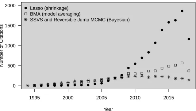
Model uncertainty can be appropriately represented if estimates from every model con-sidered are somehow accounted for (Buckland et al. 1997). Model averaging and Bayesian methods have different approaches for accounting for the various models considered (Draper 1995, Raftery 1995, Raftery et al. 1997, Hoeting et al. 1999, George and McCulloch 1993). Bayesian variable selection methods were initially proposed as a clever way to focus on promising subsets of variables without enumerating2pmodels (George and McCulloch 1993). Shrinkage techniques were developed to build predictive models more stable and with less variance than those built by the discrete process of classic variable selection methods (Tib-shirani 1996). All of these modern methods have seen rapid increase in use. Figure 2.1 shows citation frequency for three popular representatives of these modern method categories: Bayesian model averaging (BMA), Bayesian variable selection with stochastic search variable selection (SSVS), and least absolute shrinkage and selection operator (lasso). As modern methods grow in popularity, they spur adaptations for specific problems and become more computationally accessible to researchers. Application of these modern methods will only become more wide-spread. It is vital to understand how these modern methods behave in a real-data setting (George 2000).
2.7.2 Debates about Best Criterion in Sequential Analysis
1995 2000 2005 2010 2015 0
500 1000 1500 2000
Year
Number of Citations
● ●
● ●
●
●
●
●
● ●
● ● ● ● ● ● ● ● ● ● ● ● ●
● Lasso (shrinkage)
BMA (model averaging)
SSVS and Reversible Jump MCMC (Bayesian)
Figure 2.1: Citations of Modern Variable Selection Methods.
All included citations were counted on until September 10, 2018 from ISI Web of Knowledge. BMA includes citations from Raftery (1995), Raftery et al. (1997), Hoeting et al. (1999). Bayesian includes citations from George and McCulloch (1993), Green (1995). Lasso includes citations fromTibshirani (1996).
described here. First we consider the differences in AIC and BIC. A good deal of discussion exists about which criteria AIC or BIC will select the best model (Burnham and Anderson 2004). Recall AIC was derived as an approximation to the Kullback-Leibler distance between the distribution ofY as modeled in the γth model and the true distribution of Y. (Stone 1977) showed model selection with AIC is asymptotically equivalent to model selection with cross-validation. BIC was derived as an approximation to the log of the posterior probability of a model. (Schwarz et al. 1978) shows this is asymptotically equivalent to choosing a model based on Bayes factors.
identify the true model converges to 1. The same cannot be said of AIC. However, unlike AIC, BIC cannot be said to be a minimax-rate optimal estimator. This would suggest that the common practice of first selecting a best model and then drawing inference from this “best model”, could be a deeply flawed procedure. If an investigator uses AIC as the model building criterion, they would yield asymptotically good estimates of the coefficients included but could quite easily be good estimates from a seriously flawed model. Similarly, relying on BIC is asymptotically likely to land on the correct variables to include in the model, if the true model is under consideration, but could yield seriously biased estimates of coefficients. Yang (2005) nicely summarizes their investigation by stating “... when model selection instability is high, combining the models can substantially improve the accuracy of estimation/prediction. On the other hand, when the best model can be easily identified, combining the models usually loses out to model selection.”
Using p-values as criteria also has drawbacks particularly in the presence of confounders. As stated by Kleinbaum et al. (1998), testingH ∶ β2,adj =0does not address confounding, but precision. In other words, such a test evaluates whether significant additional variation inY is explained by addingC to the model. For questions of etiology, confounding likely takes precedence over precision. Also,β2 ≠0does not imply thatβ1,crude≠β1,adj. Although CIE directly assesses whetherβ1,crude ≠β1,adj, it suffers in its common use with a percent cutoff. Specifically, Lee (2014) investigates how study traits such as sample size, effect size, variance, and exposure correlation with the confounder affect what percentage cutoff would yield 80% power and 5% type I error in linear and logistic regression. Perhaps unsurprisingly, these study traits greatly affect how CIE performs demonstrating that a general rule-of-thumb cutoff should be avoided. Instead, careful examination of the traits of the study should be undertaken to better understand CIE’s operational characteristics in specific scenarios. Indeed, Lee (2014) proposes an interesting procedure to determine a situation specific cut-off.
test the relationship between explanatory variables and the outcome and proceed to a multivari-able model only with varimultivari-ables found significant in the first stage have been shown to grossly underestimate the final p-value (Viallefont et al. (2001)). Sun et al. (1996) caution strongly that this method will miss confounders which may be insignificant alone, but important to include in the model. Mickey and Greenland (1989) compare a two-stage method in the setting of a logistic regression model in a case-control study to other methods to identify confounders, in particular CIE. The two-stage methods they explore are not quite as straightforward as what we have described so far, but the conclusion drawn is the same. When confounding is present, the two-stage method too easily dismisses important variables. For the two-stage method to function adequately a higher p-value cut-off, such as 0.2, should be considered. Also, a lower percentage cut-off for CIE could also be preferable (Mickey and Greenland (1989)).
A strikingly similar conclusion is drawn in a set of simulations investigating confounder selection in Poisson models (Maldonado and Greenland (1993)). Maldonado and Greenland (1993) find that CIE performs best when the cut-point is set to a “low” 0.10, while the two-stage methods required a higher cut-off of 0.20. They further suggest the CIE estimator “...does not start to adjust for the confounder until the magnitude of confounding is about half of the cut-point value; at this degree of confounding and below, this estimator has about the same amount of bias as the crude estimator. This bias occurs even when the sample size is large, but setting the cut-point to a tolerable level of bias seems to ensure that bias will be held well below that level. For example, using a 20 percent cut-point yields a point estimator with an average bias of about 10 percent when confounding is weak.”
2.7.3 Model Uncertainty
(Draper 1995, Raftery 1995, Raftery et al. 1997, Hoeting et al. 1999). A proper accounting for the uncertainty in the actual model selection procedure needs to be incorporated to correct for this underestimation. An alternative to building the “best” single model is to fit multiple models and combine them in a sensible way. According to Hoeting et al. (1999), the idea to combine models first saw a rush of interest in the 1960s in economics journals and flourished again in the 1990s when new advancements were made and computing power was sufficient. Hoeting et al. (1999) provides a thorough history of BMA and a practical guide to BMA implementation. Madigan and Raftery (1994) note that averaging over all the models as BMA does provides better average predictive ability, as measured by a logarithmic scoring rule, than using any single model. BMA may not be a simple method to implement in every statistical analysis program, however Raftery (1995) show how to use BIC to approximate the posterior probability of a model making BMA more accessible to the analyst.
2.7.4 Previous Variable Selection Comparisons
selecting the correct model and at predicting the outcome (using the prediction score by Good). However, their simulation is limited to only 10 replications in each of two settings. All of the explanatory variables used in the simulation are independent and therefor this simulation does not address confounding. Wiegand (2010) compare backward elimination, forward selection and stepwise methods in logistic and proportional hazards setting. They particularly investigate the agreement between these methods. While many comparisons of various variable selection methods exist, comparisons of the change in effect method and Bayesian model averaging do not. Further, comparisons of stepwise regression and BMA focus heavily on which variables are included and less on how the method performs in terms of estimation and prediction.
selection methods (Rockova et al. 2012, O’Hara et al. 2009). A naive user may not understand the effects of these selections on results and rely on the suggested defaults. Non-expert’s use of variable selection methods needs careful examination to understand the actual impact of variable selection methods to applied research.
2.8 Summary
CHAPTER 3: APPLYING MODERN VARIABLE SELECTION TECHNIQUES TO A CLASSIC LINEAR REGRESSION SETTING
3.1 Introduction
Several variable selection techniques were introduced at the end of the 20th century. Com-puting advancements continue to make these methods more accessible, resulting in booming popularity for these modern methods. Simultaneous advancements in data collection, partic-ularly in the “-omics” fields, continue to encourage further development and refinement of modern variable selection techniques. Many of these modern variable selection methods were developed specifically for high-dimensional data, where the number of variables considered is significantly larger than the number of subjects. As the popularity of modern methods grows, it remains unknown how these methods behave in a classical regression model.
process. Considering multiple models and then proceeding with the selected model as if it were known to be the correct model can cause several serious problems. Variance estimates are generally underestimated, p-values are generally inflated, prediction ability is overestimated, and results are not reproducible in another dataset (Harrell 2001, Viallefont et al. 2001, Sun et al. 1996, Hurvich and Tsai 1990). In addition to causing problems with estimation and prediction, these classic variable selection methods can also lead to a final model that is not a good representation of the relationships between the variables. For example, if two variables only jointly affect the outcome, forward selection may exclude them both (Mantel 1970). Similarly, if two variables are equally explicatory of the outcome and are correlated with each other, backward elimination would only retain one of them (Mantel 1970). Lastly, classic variable selection methods may not perform well or be impossible to utilize when the number of variables,p, is large. To completely examine every model,2p models would need to be examined. Even though these short-comings were well known as long ago as the 1980s (Miller 1984, Freedman and Freedman 1983, Flack and Chang 1987, Freedman et al. 1988), classic variable selection techniques continue to be widely used (Walter and Tiemeier 2009).
1995 2000 2005 2010 2015 0
500 1000 1500 2000
Year
Number of Citations
● ●
● ●
●
●
●
●
● ●
● ● ● ● ● ● ● ● ● ● ● ● ●
● Lasso (shrinkage)
BMA (model averaging)
SSVS and Reversible Jump MCMC (Bayesian)
Figure 3.1: Citations of Modern Variable Selection Methods.
All included citations were counted on until September 10, 2018 from ISI Web of Knowledge. BMA includes citations from Raftery (1995), Raftery et al. (1997), Hoeting et al. (1999). Bayesian includes citations from George and McCulloch (1993), Green (1995). Lasso includes citations fromTibshirani (1996).
(Tibshirani 1996). All of these modern methods have seen rapid increase in use. Figure 3.1 shows citation frequency for three popular representatives of these modern method categories: Bayesian model averaging (BMA), Bayesian variable selection with stochastic search variable selection (SSVS), and least absolute shrinkage and selection operator (lasso). As modern methods grow in popularity, they spur adaptations for specific problems and become more computationally accessible to researchers. Application of these modern methods will only become more wide-spread. It is vital to understand how these modern methods behave in a real-data setting (George 2000).
non-high-dimensional setting. First, all of these studies only report variable selection method performance in terms of prediction abilities and/or variable selection characteristics and do not report estimation capabilities. Second, most of these studies assume predictor variables are either uncorrelated or have a very simple correlation structure. Independent variables or minimal correlation is unlikely to appear in non-high-dimensional practice. Third, all of these studies report simulations based on 100 or fewer subjects. A few other studies show compar-isons of some modern methods highlighted here in the non-high-dimensional setting (Swartz et al. 2008, Viallefont et al. 2001, Genell et al. 2010). In addition to lacking comparisons between all the methods of interest here, SSVS, BMA and adaptive lasso, these also fail to report on the quality of estimation (e.g., bias, coverage, etc.) of the variable selection methods. Finally, previous simulation studies have examined effects of various priors, tuning parameters, cut-offs and computational specification to understand how to maximize the capabilities of selection methods (Rockova et al. 2012, O’Hara et al. 2009). A naive user may not understand the effects of these selections on results and rely on the suggested defaults. Non-expert’s use of variable selection methods needs careful examination to understand the actual impact of variable selection methods to applied research.
The study presented here compares estimation, prediction, and variable selection perfor-mance among modern variable selection methods, specifically BMA, SSVS and adaptive lasso. This study also includes comparisons to classic variable selection techniques. These methods are applied to linear regression in a study where a single variable of interest exists in the presence of possible confounding. A variety of sample sizes ranging from 150 to 20,000 are investigated. Freely available and easily executable methods with default tuning parameters and simple priors are used to mimic use by non-expert users.
The simulation design follows in Section 4 with simulation results described in Section 5. Section 6 summarizes the detailed results presented in Section 4. Lastly, summary conclusions are made in the final section.
3.2 Background and Review of Representative Modern Variable Selection Methods
This simulation study focuses on the application of variable selection in a linear model. Linear models are employed to investigate the relationship between the response,Yiand thep possible explanatory variablesxi0, . . . , xip. Assume there arensubjects,i=1. . . , n. A linear model is of the form
Yi =β0+β1Xi1+. . .+βpXip+i (3.1)
i ∼N(0, σ2) (3.2)
Note,Xi1, . . . Xip, could also be nonlinear functions. The predicted values ofY are denoted by and are defined as
ˆ
Yi =βˆ0+βˆ1Xi1+. . .+βpXipˆ (3.3)
In classical linear regression theβˆj minimize the squared error, also called the residual sum of squares, RSS.
Many modern variable selection methods exist. Three representative methods are studied in this paper and are described below along with a brief description of the classic methods.
3.2.1 Bayesian Model Averaging
model averaging (BMA) provides an opportunity for exploring many possible models while appropriately accounting for the uncertainty surrounding variable selection (Draper 1995, Raftery 1995, Raftery et al. 1997, Hoeting et al. 1999). BMA is only one of several statistical methods developed for appropriately accounting for model uncertainty but has the advantage of providing optimal predictive performance (George 2000, Madigan and Raftery 1994). Madigan and Raftery (1994) measured predictive performance in a logistic regression model using a logarithmic scoring rule. However, given their reported lack of use, BMA methods are either unknown or not easily accessed by many researchers (Walter and Tiemeier 2009).
Bayesian model averaging performs inference using a weighed average of model-specific results from all the models considered. Consider the setting where a researcher has a proposed (finite) class of modelsM. Suppose that∆is a quantity of interest, such as a predicted value of a future observation or an effect estimate, and that the set of proposed modelsM contains as elements the modelsM1, . . . , MK. Then the posterior distribution given dataDis defined by the following weighted average
p(∆∣D) = K ∑ k=1
p(∆∣Mk, D)p(Mk∣D). (3.4)
If the model building goal includes understanding the relationships between variables, it can be helpful to know the probability that each model is correct. It is convention to refer to p(Mk∣D), or the probability modelMkis correct given the observed data, as the Posterior Model Probability (PMP).
p(Mk∣D) =
p(D∣Mk)p(Mk) ∑K
h=1p(D∣Mh)p(Mh)
(3.5)
where
p(D∣Mk) =
ˆ
vector of the form(β′, σ2)′. BMA constructs a weighted-average model by using PMP as the weights. Another very useful posterior probability from this process is the posterior inclusion probability, or PIP. PIP is the probability of a variable appearing the true model and can be found by summing the PMP’s of all models which include the variable. PIP can also be thought of asP(βj ≠0∣D).
BMA requires the user to definep(Mj), also called the prior model probability. This allows the researcher to place heavier weight on models which are deemed more likely. If there is not information available to inform this decision, each model can be assumed to be equivalently likely, or each variable could be assumed to have a 50% chance of being included.
While some settings allow for a completely Bayesian approach to model averaging, the BMA approach taken in this paper is one that is more widely applicable across settings which differ in model type and number of parameters considered. This study applies the BIC approximation presented in Raftery for the integral in (4.7) (Yeung et al. 2005, Raftery 1995). Instead of enumerating every possible model, it has been argued that it more closely mirrors the scientific process to restrict the model set (Madigan and Raftery 1994, Raftery et al. 1997). The Occam’s window approach used in this paper excludes models from consideration that are significantly less likely than the most likely model and/or contain sub-models which are dramatically more likely (Hoeting et al. 1999). In settings with many variables, Occam’s window is a less computationally intensive option. See Hoeting et al. (1999)for a thorough history of BMA and a practical guide to BMA implementation.
3.2.2 Stochastic Search Variable Selection (SSVS)
variable,γj, whereP(γj =1) =πj. The mixture distribution forβj is
βj∣γj ∼ (1−γj)N(0, τj2) +γjN(0, c2jτ 2
j). (3.7)
Selectingτj to be a small positive number andcj a large number greater than 1, ensures that whenγj =0,βj is likely to be zero and whenγj =1,βj is unlikely to be zero. In this way,πj can be thought of as the prior probability that variableXj should be included in the model (George and McCulloch 1993). The above can be achieved with a multivariate normal prior
β∣γ ∼Np(0,DγRDγ) (3.8)
whereγ = (γ1, ...γp),Ris the prior correlation matrix, and
Dγ =diag[a1τ1, ..., apτp] (3.9)
withai=1ifγi=0andai=ciifγi=1. An inverse gamma prior is used forσ2∣γ,
σ2∣γ ∼IG(νγ
2 ,
νγλγ
2 ). (3.10)
Using the interpretation thatνγis the number of observations and νγ
(νγ−2)λγis the estimate of σ2 in an imaginary previous experiment can be helpful in selecting the hyper-parameters. For a detailed discussion about all the prior specifications, see George and McCulloch (1993).
When introduced, the authors cautioned that SSVS may be slow to converge if multiple models had high posterior probability. This can frequently happen when variables are collinear. They suggest eliminating collinearities before using SSVS, or performing two rounds of selection this first using SSVS and the second using SSVS again or backward elimination (BE) (George and McCulloch 1993). The two-round selection is not employed here.
3.2.3 Adaptive Lasso
Ridge regression, lasso and adaptive lasso all seek a model which minimizes a penalized residual sum of squares (RSS) by simultaneous estimation and variable selection. Ridge regression penalizes with a tuning parameter,λ, multiplied by the sum of the squared coef-ficients and the lasso penalizes with a tuning parameter times the sum of the absolute value of the coefficients (Tibshirani 1996). While ridge regression can shrink estimates, it cannot eliminate them from the model by forcing the estimates to be zero thereby simplifying the results. Lasso was developed as a way to combine the shrinkage idea in ridge regression and the selection idea of best subsets to both improve predictive performance and simplify the model(Tibshirani 1996). The adaptive lasso generalizes the lasso by using a penalty which allows weights to be applied to the absolute value of the coefficients as follows (Zou 2006).
RSS(β) +λ p ∑ j=1
ˆ
wj∣βj∣ (3.11)
Unlike the lasso, adaptive lasso has what is known as an oracle property, meaning, under certain conditions, and asnincreases the adaptive lasso will find the correct model (Zou 2006). Adaptive lasso is selected in this study to allow investigation of the setting where there is a particular variable of interest that must be included in every model. By settingwj =0for the variable of interest, inclusion is guaranteed (Friedman et al. 2010). See Hastie and Qian for an introduction to running these computationally intensive procedures withglmnetpackage in
Since introduction, the lasso has provided a computationally efficient approach for ex-ploring large sparse data (Tibshirani 2011). However, Tibshirani acknowledges that it is difficult to obtain standard error estimates from the lasso (Tibshirani 1996). Zou suggests an approximation for standard errors with adaptive lasso. Zou’s approximation is not easily implemented. Chatterjee et al. (2013) suggest using residual bootstrap methods. To mimic use by a non-expert user, neither are included in this study.
3.2.4 Classical Variable Selection Methods
For the purposes of understanding how modern variable selection techniques behave in a non-high-dimensional regression setting, classic variable selection techniques are also included in the simulation. Popular classic variable selection methods include forward selec-tion, backward eliminaselec-tion, stepwise, best-subset, and two-phase (all significant univariate relationships included in a multivariate model) (Walter and Tiemeier 2009). Classical variable selection techniques have been described and compared in detail elsewhere (Mantel 1970, Miller 2002, Mickey and Greenland 1989, Sun et al. 1996, Viallefont et al. 2001). It is known that backward elimination is more appropriate than forward or step-wise in settings with collinearity (Mantel 1970). This study evaluates BE with selection criteria of AIC, BIC, p=0.05 and p=0.20, however for simplicity, only BE with BIC is shown. BE with BIC was found to be the least likely of these to suffer from an underestimate of model uncertainty in our full simulation and behaved similarly to BMA in regards to variable selection.
3.3 Motivating Example
random cluster design, a stratified probability sample was used to select counties and cities stratified by income and urbanization. Communities and households were then randomly selected from these strata. Survey procedures have been described elsewhere (Popkin 2010). The study was approved by the Institutional Review Board at the University of North Carolina at Chapel Hill, the China-Japan Friendship Hospital, the Ministry of Health and China, and the Institute of Nutrition and Food Safety, China Centers for Disease Control. Participants gave informed consent.
For the purposes of demonstrating the traits of variable selection methods, this paper considers the specific goal of modeling whether waist-to-height ratio greater is than 0.5 among participants who were surveyed in at least two rounds while they were between the ages of 18 and 30 and have their waist circumference and height recorded. After excluding all missing data, N=1195. The specific variable of interest is a measure of urbanization and potential explanatory variables include the following: age, sex, income, years of education, physical activity, caloric intake, sodium, potassium, whether the participant smokes, whether the participant consumes alcohol, and whether the participant drinks coffee. Coffee drinking was included because it was highly correlated to urbanization, but was not believed to be related to waist-to-height ratios. Although perhaps unlikely to be included in an actual research setting, coffee drinking was included to investigate how the model selection methods would handle this type of relationship between variables. The simulation study generates data meant to mimic this example. All explanatory variables were standardized. The correlation between the explanatory variables, the effect sizes, and the error variance found in the example data guide the simulation parameters.
3.4 Design of the Simulation Study
less than 0.7% for a proportion, such as the probability of including a variable (Koehler et al. 2009).
3.4.1 Data Generation
Table 3.1: Explanatory Variable Correlations for Data Generation.
XIN T EREST X1,EC X2,C X3,C X4,C X5 X6 X7,C B8 B9,E B10 B11,EC
XIN T EREST 1 0.1 0.2 -0.5 -0.2 0.5 0.2
X1,EC 0.1 1 0.2 -0.1 0.2
X2,C 0.2 1 -0.1 -0.1 0.2 0.1
X3,C -0.5 0.2 -0.1 1 0.1 -0.4 -0.1
X4,C -0.2 -0.1 0.1 1 0.4 0.6 -0.1 0.2 0.2 -0.3 -0.1
X5 -0.1 0.4 1 0.3
X6 0.6 0.3 1 0.1 0.1 -0.1
X7,C 0.5 0.2 -0.4 -0.1 1 0.1 -0.1 0.2
B8* 0.2 0.1 1 0.5 -0.5
B9,E* 0.2 0.1 0.1 0.5 1 -0.4
B10* 0.2 -0.3 -0.1 -0.1 -0.5 -0.4 1 0.1
B11,EC* 0.2 0.1 -0.1 -0.1 0.2 0.1 1
*
Some of the variables are transformed from normally distributed variables into binary variables with a cut point determined at a random quantile. For example, it is desired that on average 25% of observations have B8 =1. At each replication of the simulation a cut point varied uniformly between 20% and 30% to achieve an average of 25%. Desired observed proportions forB8 throughB13are 0.25, 0.25, 0.5,0.05, 0.7, and 0.3 respectively.
Four variables,B12,B13,E,X14,X15,E are uncorrelated with all other variables and are not included here.
Lastly, the outcome variable is generated in the following manner:
Y =0.45+0.01XIN T EREST +0.01X1,EC−0.01B9,E−0.01B11,EC+0.005B13,E+ (3.12)
0.005X15,E+
Sample sizes ofn=150,250,500,1000,2500,5000,10000,and20000are investigated. Error is distributed normally with mean of zero and variance of 0.0016 for alln, resulting in an r2 ∼0.13. Whenn=1000, error variances of .0625, 0.01 and 0.0004 are also considered in order to investigate models with higher and lower predictive abilities than what was observed in the CHNS example. These error variances result inr2 of approximately 0.40, 0.03, and 0.01 respectively. Also for the setting ofn=1000, the situation where the variable of interest has no effect is considered. Although this data is more complicated than is generally reported in simulations comparing variable selection methods, it is a more accurate depiction of the conditions of a large observational study (Wang et al. 2004, Wiegand 2010, Lee 2014). A table outlining the full design of the simulation study is available in the supplemental material, Table A.1.
3.4.2 Variable Selection
final models, the coefficient estimates, the standard error estimates and predicted values of the outcome for these selected models are recorded. BMA and SSVS provide averaged estimates of coefficients, standard errors and predicted values of the outcome which are also recorded. For BMA and SSVS, PMP and PIP values for each replication are recorded. Lastly, coefficient estimates from the final model or the averaged model from each method are applied to the last nof the2nobservations and predicted outcomes are recorded.
3.4.3 Quantities of Interest
Model Selection and Variable Inclusion Probabilities
The first of four key modeling aims this simulation will investigate is selecting the correct model. The model selected by each procedure is recorded, and the probability of selecting any particular model is the number of replications selecting a specific model and dividing by r, here 1000. Because so many variables are examined, the variety of models chosen by the selection methods considered here are well over 1000. For this reason, the models selected are summarized by determining if they select all, some or none of the variables withβ≠0
(X1,EC, B9,E,B11,EC, B13,E, andX15,E),and all, some, or none of the variables related to XIN T EREST but withβ=0(X2,C,X3,C,X4,C, andX7,C). These two groups are referred to as the E group, for effect, and the C group, for correlated. Note, the true model includes only the E group. Ideally the methods will select the true model, but if that cannot be achieved, the model should at least include all of the E group.
Additionally, the variable inclusion probabilities (IP) are presented. For all methods except BMA and SSVS, IP is the percent of simulation replicates selecting each variable in the final model. Average PIP across replications is reported for BMA and SSVS. The individual variable’s IP are essential for understanding how these selection methods function with variables that differ in effect size, correlation, and type (binary vs. continuous). If the true model is not selected, these IP can help determine why.
Estimation of Main Effect
include this variable. The bias, standard error of the coefficient estimates, ratio of the standard deviation of the coefficient estimates and the mean estimated standard error, coverage, and the probability of type I error or power, depending on the scenario, are recorded. The ratio of the standard deviation of the coefficients and the mean estimated standard deviation is a measure of how well methods account for model uncertainty. The standard deviation of the coefficients reflects the variance of the coefficient estimate including the variance attributed to the uncertainty in the model selection process. The mean of the standard error estimates represents the value likely to be reported by a researcher using a variable selection technique. If this ratio is greater than 1, the reported standard deviations are too small which in turn results in overly optimistic p-values.
Predictive Performance
The third modeling goal is predicting the outcome. Predictive performance is measured by the Pearson correlation between the predicted values ofY and the actual values ofY,ρY
orig,Yˆ,
in the simulated original and external datasets. The difference between these two correlations reveals a degree of over-fitting,ω(Harrell 2001).
ˆ
Yorig=Xorigβorigˆ (3.13)
ˆ
Yexternal=Xexternalβˆorig (3.14) ω=ρY
orig,Yˆorig−ρYexternal,Yˆexternal (3.15)
The ideal model has the highestρY
external,Yˆexternal and the lowestω. Negativeωwould indicate
Agreement
Agreement is not really a modeling goal but aids our understanding of how these methods relate to each other. The fourth and final quantity investigated is the probability that these variable selection strategies agree with each other. With so many variable selection methods available, one suggested technique is to perform multiple methods and declaring a model final if it is chosen by both methods (Wiegand 2010). Investigating method agreement will also highlight the similarities between the selection methods.
3.5 Simulation Results
3.5.1 Model Probabilities
0 5000 10000 15000 20000 0.0
0.2 0.4 0.6 0.8 1.0
n
P
ercent of Replicates Selecting Correct Model
1000
SSVS Top SSVS Median BE BIC BMA BIC Top BMA BIC Median
Adaptive Lasso
Figure 3.2: Probability of Selecting the True Model.
Figure 3.2 shows the probability that each method reports the model that contains all variables withβ≠0with no other variables. Adaptive lasso struggles to findB11,EC, the only variable with an effect in the opposite direction of its correlation withXIN T EREST.
3.5.2 Variable Probabilities
Variable IP for a subset of the sample sizes is shown in Figure 3.3. The variables have been arranged with the most important group at the top, variables with both an effect and a correlation withXIN T EREST and haveECas a subscript. These are followed by variables with an effect but no correlation (Esubscript), variables with correlation but no effect (Csubscript), and lastly variables with neither an effect nor a correlation (noise, no subscript). Other noise variables are not shown in the plot. The noise variables shown here had no correlation with the variable of interest and no correlation with any other variables considered. Also not shown are the IP from SSVS and BMA top and median models. The top and median models closely match their corresponding averages for IP. Variable IPs vary considerably not only by method but also by the variable effect size, potential correlation withXIN T EREST, variable type (continuous or binary), and sample size. Complete tables of inclusion probabilities for n=1000andn=20000can be found in the appendix.