STRUCTURAL AND SPATIAL ANALYSIS OF THE MICROBIAL COMMUNITIES IN SOIL CONTAMINATED WITH POLYCYCLIC AROMATIC HYDROCARBONS
Juliet S. Swanson
A dissertation submitted to the faculty of the University of North Carolina at Chapel Hill in partial fulfillment of the requirements for the degree of Doctor of Philosophy in the
Department of Environmental Sciences and Engineering. Chapel Hill
2007
Approved by
ABSTRACT Juliet S. Swanson
STRUCTURAL AND SPATIAL ANALYSIS OF THE MICROBIAL COMMUNITIES IN SOIL CONTAMINATED WITH POLYCYCLIC AROMATIC HYDROCARBONS
Under the direction of Frederic K. Pfaender.
The microbial communities of an aged, creosote-contaminated soil (CMN) and an uncontaminated soil (PMN) from nearby were compared. Polymerase chain reaction (PCR) amplicons of small subunit ribosomal RNA-encoding genes were resolved on a denaturing gradient gel (DGGE) and transformed into clone libraries. The CMN community was less diverse than the PMN, as evidenced by 1) the finite number of DGGE bands versus the smeared profile of the PMN and 2) the finite number of unique clones versus the flat rank abundance of the PMN clones. The CMN clone library contained sequences belonging only to the Proteobacteria, whereas the PMN sequences represented numerous phylotypes.
association of cells and pyrene with soil particles in the slurried samples. Other patterns also emerged: 1) the higher the background PAH contamination, the more cells clustered with respect to pyrene, and 2) the clustering tendency increased over time for the least
contaminated soil and decreased for the others. These data suggest that better-adapted populations are present in more contaminated soils.
The change in the bacterial community structure of the spiked PMN was monitored by PCR-DGGE. The PMN profile became less diverse over time but never approached that of the CMN, even after an additional pyrene spike. The community did not recover its original diversity, indicating either permanent succession or an ongoing selection of certain
ACKNOWLEDGMENTS
This research was funded by the Superfund Basic Research Program and the National Institutes of Environmental Health Sciences (Grant No. 5 P42 ES 05948).
I would like to thank all the members of my doctoral committee for their guidance, patience, and insight. I am grateful to the Pfaender/Aitken lab group members for their commiseration in the face of unsuccessful experiments and their assistance with my infamous lack of computer skills.
DEDICATION
TABLE OF CONTENTS
1.0 Introduction………...1
1.1 Scope and Objectives...3
1.2 Significance...4
2.0 Literature Review………...……….6
2.1 Microbial Diversity and rRNA Phylogeny………...6
2.2 Characterizing Microbial Diversity: the Application of Molecular Methodology to Environmental Samples...8
2.2.1 Culture-based versus culture-independent methods...8
2.2.2 Nucleic acid extraction from soils...10
2.2.3 rRNA-dependent methodologies: advantages and disadvantages of PCR, DGGE, and FISH...12
2.3 Factors Influencing Microbial Community Development and Diversity in Soil...20
2.3.1 Soil type...20
2.3.2 Soil organic matter...21
2.3.3 Cultivation effects...21
2.3.4 Terminal electron acceptors...22
2.3.5 Seasonal variation and spatial isolation...23
2.3.6 Microbial communities in soil...24
2.4.1 Resistance and resilience...25
2.4.2 Examples from literature...27
2.5 General Background on PAHs: Sources, Properties, Fate, and Health Effects...33
2.5.1 Sources...33
2.5.2 Properties affecting fate...33
2.5.3 Health effects...35
2.6 Factors Affecting Contaminant Bioavailability...36
2.6.1 Soil characteristics………...……36
2.6.1.1 Physico-chemical characteristics...36
2.6.1.2 Organic carbon content and character...38
2.6.1.3 Sequestration...39
2.6.2 Microbial characteristics………...……40
2.6.2.1 Adhesion and biofilms...40
2.6.2.2 Motility and chemotaxis...40
2.6.2.3 Substrate uptake...41
2.6.2.4 Cell surface hydrophobicity and biosurfactant production…………...41
2.7 Factors Affecting Biodegradation Rates...43
2.7.1 Prior exposure...43
2.7.2 Degrader numbers...43
2.7.3 Substrate competition...44
2.7.4 Presence of inducers...44
2.7.6 Presence of fungi...45
2.7.7 Plant presence...46
2.8 Microbial Metabolism of PAHs, Specifically Pyrene...46
2.8.1 General aerobic...46
2.8.2 General anaerobic...48
2.8.3 Pyrene transformation...48
2.8.4 Genes involved in PAH degradation...51
3.0 Comparison of the Microbial Communities in an Aged, PAH-Contaminated Soil and an Uncontaminated Soil from within the Same Site………...……….54
3.1 Introduction……….54
3.2 Materials and Methods………...56
3.2.1 Soils………...……56
3.2.2 DNA extraction………..57
3.2.3 Polymerase chain reactions (PCR)……….58
3.2.4 Denaturing gradient gel electrophoresis (DGGE)………...……...59
3.2.5 Clone libraries………...…….60
3.2.6 DNA sequencing………...…….60
3.2.7 Sequence analysis………..60
3.2.8 Diversity analysis………...61
3.3 Results……….62
3.3.1 DGGE………...62
3.3.2 Clone libraries and phylogenetic trees………...65
3.4 Discussion………...75
3.4.2 Diversity measurements……….77
3.4.3 Species loss………...78
3.4.4 Archaea………..80
3.4.5 Reasons for changes in the CMN structure………...80
3.4.6 Anaerobic effects………...83
3.4.7 Storage effects………84
3.5 Method Limitations……….……84
3.6 Future Research………..86
4.0 Comparison of a Slurry-based Method and an Aggregate Method for the in situ Visualization of Microorganisms in PAH-contaminated Soils………...88
4.1 Introduction……….88
4.2 Materials and Method Optimization………...91
4.2.1 Soils………...91
4.2.2 Chemicals and reagents………..91
4.2.3 Probes……….92
4.2.4 Filter apparatus………...92
4.2.5 Microscopy………93
4.2.6 Image processing and analysis………...94
4.2.7 Statistics……….94
4.3 Method Optimization………..94
4.3.1 Choice of fluorochrome……….94
4.3.2 The embedding method………..97
4.3.2.1 Sample preparation by embedding………97
4.3.2.3 Validation of the embedding method………98
4.3.3 Optimization of hybridization buffer composition and pH, wash solution strength and pH……….…………..101
4.4 Method Validation: Fluorescence in situ Hybridization of Cells in PAH-Contaminated Soils Spiked with Pyrene and Subsequent Examination of Spatial Relationships Therein………104
4.4.1 Spiking procedure………104
4.4.2 Sample preparation and fixation………..105
4.4.3 Sample pretreatment………106
4.4.4 Hybridization………...106
4.4.5 Washing………...106
4.4.6 Microscopy and image acquisition………..106
4.4.7 Image processing……….106
4.4.8 Image analysis………..109
4.4.8.1 Cell enumeration……….109
4.4.8.2 Pyrene prevalence………...109
4.4.8.3 Overall object distribution………..109
4.4.8.4 Distribution of cells with respect to pyrene………110
4.4.9 Results and discussion of method validation test………112
4.4.9.1 Cell enumeration: plate counts, Slurry FISH and Aggregate FISH counts………112
4.4.9.2 Pyrene prevalence………...117
4.4.9.3 Object distribution………..119
4.4.9.3.1 Dispersion indices………..119
4.4.9.4 daime: spatial arrangement analysis of cells and pyrene…………...122
4.4.9.4.1 Pair cross-correlation values………..122
4.4.9.4.2 Frequency distributions of nearest neighbor values………...128
4.4.9.5 Summary of spatial arrangement analyses………..135
4.5 Method Limitations…..……….136
4.6 Conclusions..……….138
5.0 The Change in Microbial Community Structure over Time in a Previously Uncontaminated Soil Spiked with Pyrene………...141
5.1 Introduction..……….141
5.2 Materials and Methods..………145
5.2.1 Soils..………...145
5.2.2 Chemicals and reagents...……….146
5.2.3 Oligonucleotide synthesis…..………..146
5.3 Experimental Methods………..………147
5.3.1 Microcosm set-up and incubation…..………..147
5.3.1.1 Respiking………..………..149
5.3.2 “Hot” microcosm sampling: 14C-pyrene measurements……..…………...149
5.3.3 “Cold” microcosm sampling: DNA extraction, PCR-DGGE, Quantitative PCR, plate counts, and FISH………..………...150
5.3.3.1 DNA extraction…..……….150
5.3.3.2 Polymerase chain reaction-denaturing gradient gel Electrophoresis (PCR-DGGE)……..………...150
5.3.3.3 Quantitative polymerase chain reaction (qPCR)..………...151
5.3.3.4 Plate counts..………...152
5.3.3.6 Microscopy and image acquisition..………...153
5.3.3.7 Image processing..………..154
5.3.3.8 Image analysis…..………...155
5.3.4 Statistical analyses..……….158
5.4 Results and Discussion………..………...159
5.4.1 14C-Pyrene compartmentalization..………..159
5.4.1.1 Mineralization..………...159
5.4.1.2 Aqueous phase-associated radioactivity……….163
5.4.1.3 Solid phase-associated radioactivity………...166
5.4.1.4 Respiked microcosms..………...166
5.4.1.5 Mass balance of pyrene..……….170
5.4.2 Plate counts and direct cell counts..……….171
5.4.3 Community diversity comparisons: DGGE profiles..……….176
5.4.4 Appearance of pyrene degraders..………182
5.4.5 Presence or absence of pyrene..………...188
5.4.6 Object distribution and spatial analyses..……….190
5.4.6.1 Dispersion indices..……….190
5.4.6.2 Nearest neighbor analysis: cell to cell and/or pyrene..………..190
5.4.6.3 daime: spatial arrangement analysis of cells and pyrene..……….195
5.4.6.3.1 Pair cross-correlation values..………195
5.4.6.3.2 Frequency distributions of nearest neighbor values..……….201
5.5 Conclusions…..……….207
LIST OF TABLES
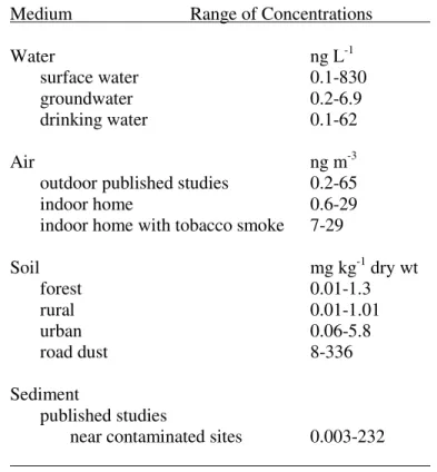
2.1. PAH-degrading Organisms Isolated from Enrichment Cultures...32
2.2. Measured PAHs in a Sampling of Different Environmental Media and Geographical Locations………..34
2.3. Levels of EPA-PAHs in Temperate Soils by Soil Type……..………34
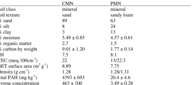
3.1. Characteristics of Experimental Soils...………...57
3.2. Primers for the PCR Amplification of Extracted Soil DNA………58
3.3. Results of rRNA Gene Sequence Analysis of DGGE Bands..………..………..67
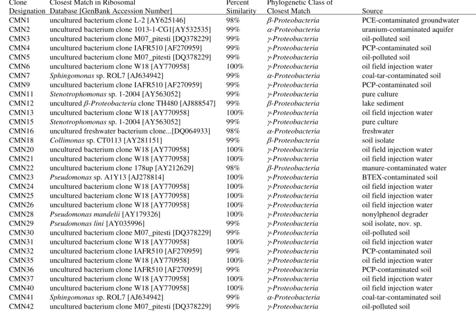
3.4. Results of CMN Clone Library………....68
3.5. Results of PMN Clone Library………....71
4.1. Characteristics of Experimental Soils………...91
4.2. Cell Counts for Each Soil Over Time, as Determined by R2A Plate Counts and Slurry and Aggregate FISH Counts, using both Univ1390-FITC and Eub338-TRITC………...112
4.3. Pyrene Prevalence………...117
4.4. Dispersion Indices Based on Cell Counts for Each Image……….…………...120
4.5. Observed/Expected Ratios of Mean Nearest Neighbor Values…………...………...121
4.6. Average Pair Correlation Values (± standard deviation) and the Percentage of Values Exceeding 1 for the CMN Soil at a Given Distance from Pyrene. Comparison of Each FISH Method at Each Time Point………...123
4.7. Average Pair Correlation Values (± standard deviation) and the Percentage of Values Exceeding 1 for the CNC Soil at a Given Distance from Pyrene. Comparison of Each FISH Method at Each Time Point………...125
4.8. Average Pair Correlation Values (± standard deviation) and the Percentage of Values Exceeding 1 for the KKY Soil at a Given Distance from Pyrene. Comparison of Each FISH Method at Each Time Point………….…...127
5.2. Oligonucleotides for PCR Primers and FISH Probes………...………...147
5.3. Comparison of Mineralization Data for CMN, PMN, and Respiked PMN…..……...162
5.4. Similarity Matrix of Sorensen’s Similarity Coefficients Calculated from a Pair-wise Comparison of DGGE Banding Patterns…..………..…...180
5.5. Pyrene Prevalence in FISH Images………....188
5.6. Indices of Dispersion for Replicate Microcosms………..……...190
5.7. Observed/Expected Ratios of Mean Nearest Neighbor Values………...191
LIST OF FIGURES
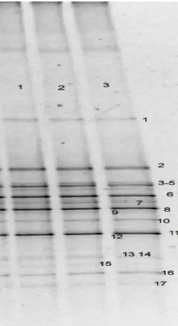
2.1. Proposed Pathways for the Microbial Transformation of Pyrene...49 3.1. DGGE Profile of Bacterial Amplicons from CMN. Lanes 1-3
represent replicate DNA extraction protocols……….…………...62 3.2. Bacterial Profile of CMN and Dilutions of PMN. Shared bands are
Highlighted. Lanes -1 through -6 represent dilutions 10-1 through 10-6
of the original PMN extract prior to PCR-DGGE………...63 3.3. Archaeal DGGE Profile of Both PMN (lane 1) and CMN (lane 3) Soils
Lane 2 is a PMN duplicate with half the template mass loaded onto the gel……...64 3.4. DGGE Profile of Fungal PCR products from PMN………...65 3.5. Phylogenetic Tree Inferred from CMN Clone Library. Mycobacterium
vanbaalenii is included as an outgroup from which the tree is rooted. Also included are reference sequences most closely related to the CMN clones. Solid circles indicate greater than 70% bootstrap support;
open circles indicate greater than 95% bootstrap support………...70 3.6. Phylogenetic Tree Inferred from PMN Clone Library. Bacillus cereus
is included as an outgroup from which the tree is rooted. Also included are reference sequences most closely related to the PMN clones.
Solid circles indicate greater than 70% bootstrap support; open circles
Indicate greater than 95% bootstrap support………...73 3.7. Phylogenetic Tree Inferred from both CMN and PMN Clone Libraries………...74 3.8. Rank Abundance Plot for CMN Clone Library………...76 3.9. The Distribution of Clones/DGGE Bands Across Common Soil
Phylotypes. Blue: PMN clones; fuschia: CMN clones; beige: CMN
DGGE bands...………...77 3.10. Rarefaction Curves of Observed OTUs in PMN and CMN Soils
Blue: PMN clones; green: CMN clones………...86 4.1. Miller-Scholin Apparatus for Filter-based Hybridizations…………...…………...93 4.2. Autofluorescence of CMN Soil. Soil smears in water were visualized
using the following filters: a) FITC, b) TRITC, c) Cy 3 ex. 520, em. 570,
4.4 a and b. Enumeration of DAPI-Stained Cells at Four Core Depths for Duplicate Embedded Cores, A and B. Introduction of acrylamide
begins at Arbitrary Core Depth 1.………...100 4.5. Example of Image Reduction: Extraction of Objects from KKY
Slurry FISH Images Taken with (a) TRITC filter to show cells and (b) PYR filter showing pyrene and added together to produce (c)
the reduced image………..……….……...108 4.6. Illustration of daime Stereological Analysis. (a) A radius, r, from
the center of a bacterial cell (red), is defined over a range. Pyrene crystals (blue) within this radius will be “hit” by a dipole of that length. (b) Hits are shown with a solid line, misses with dashed lines
(from Daims et al., 2006)………...111 4.7a. Comparison of Cell Counts in the CMN Soil Obtained by Plating,
Slurry FISH, and Aggregate FISH. Separate Results are provided for each Probe. Blue: CFU; magenta: Slurry FISH Univ1390; beige:
Slurry FISH Eub338; aqua: Aggregate FISH Univ1390; purple: Aggregate
FISH Eub338.………...113 4.7b. Comparison of Cell Counts in the CNC Soil Obtained by Plating,
Slurry FISH, and Aggregate FISH. Separate Results are provided for each Probe. Blue: CFU; magenta: Slurry FISH Univ1390; beige:
Slurry FISH Eub338; aqua: Aggregate FISH Univ1390; purple: Aggregate
FISH Eub338.……….………...113 4.7c. Comparison of Cell Counts in the KKY Soil Obtained by Plating,
Slurry FISH, and Aggregate FISH. Separate Results are provided for each Probe. Blue: CFU; magenta: Slurry FISH Univ1390; beige:
Slurry FISH Eub338; aqua: Aggregate FISH Univ1390; purple: Aggregate
FISH Eub338.………...114 4.8a. Cross-Correlation Values Calculated over Distance: A Comparison
of Slurry FISH versus Aggregate FISH for CMN at Week 2. Blue: Aggregate FISH g(r) values; pink: Slurry FISH g(r) values; aqua
dotted line: random distribution.………...122 4.8b. Cross-Correlation Values Calculated over Distance: A Comparison
of Slurry FISH versus Aggregate FISH for CMN at Week 7. Blue: Aggregate FISH g(r) values; pink: Slurry FISH g(r) values; aqua
dotted line: random distribution.……….…...123 4.9a. Cross-Correlation Values Calculated over Distance: A Comparison
Aggregate FISH g(r) values; pink: Slurry FISH g(r) values; aqua
dotted line: random distribution.………...124 4.9b. Cross-Correlation Values Calculated over Distance: A Comparison
of Slurry FISH versus Aggregate FISH for CNC at Week 7. Blue: Aggregate FISH g(r) values; pink: Slurry FISH g(r) values; aqua
dotted line: random distribution.………..…...125 4.10a. Cross-Correlation Values Calculated over Distance: A Comparison
of Slurry FISH versus Aggregate FISH for KKY at Week 2 Blue: Aggregate FISH g(r) values; pink: Slurry FISH g(r) values; aqua
dotted line: random distribution.. ………...126 4.10b. Cross-Correlation Values Calculated over Distance: A Comparison
of Slurry FISH versus Aggregate FISH for KKY at Week 7. Blue: Aggregate FISH g(r) values; pink: Slurry FISH g(r) values; aqua
dotted line: random distribution.………...…………...127 4.11a. Nearest Neighbor Distribution versus Distance: A Comparison of
Slurry FISH versus Aggregate FISH for the CMN Soil at week 2
Pink: Aggregate FISH; green: Slurry FISH……….…………...129 4.11b. Nearest Neighbor Distribution versus Distance: A Comparison of
Slurry FISH versus Aggregate FISH for the CMN Soil at week 7
Pink: Aggregate FISH; green: Slurry FISH……….…………...129 4.12a. Nearest Neighbor Distribution versus Distance: A Comparison of
Slurry FISH versus Aggregate FISH for the CNC Soil at week 2
Pink: Aggregate FISH; green: Slurry FISH………...131 4.12b. Nearest Neighbor Distribution versus Distance: A Comparison of
Slurry FISH versus Aggregate FISH for the CNC Soil at week 7
Pink: Aggregate FISH; green: Slurry FISH………...132 4.13a. Nearest Neighbor Distribution versus Distance: A Comparison of
Slurry FISH versus Aggregate FISH for the KKY Soil at week 2
Pink: Aggregate FISH; green: Slurry FISH……….…………...133 4.13b. Nearest Neighbor Distribution versus Distance: A Comparison of
Slurry FISH versus Aggregate FISH for the KKY Soil at week 7
Pink: Aggregate FISH; green: Slurry FISH……….…………...134 5.1. Pyrene Mineralization Curve. Measurements shown are the average
and standard deviation of multiple replicates. Blue: sample microcosms;
5.2. Aqueous Phase-associated Radioactivity. Blue: sample; pink: control. Sample measurements shown are the average of duplicate microcosms. Error bars represent the range. Control
measurements were not replicated ………...164 5.3. Solid Phase-associated Radioactivity. Blue: sample; pink: control. Sample
measurements shown are the average and standard deviation of triplicate subsets from each of duplicate microcosms. Control measurements are the average and standard deviation of triplicate subsamples from within a singular microcosm. Error bars are given in one direction only for ease
of reading at the earlier time points.……….…...166 5.4. Mineralization Curve for Respiked Pyrene. Blue: sample; pink: control.
Measurements shown are the average and standard deviation of multiple
replicates.………...167 5.5. Aqueous Phase-associated Radioactivity in Respiked Microcosms. Blue:
sample; pink: control. Measurements shown are the average and range
of duplicate microcosms. Control microcosms were not replicated.………...…...168 5.6. Solid Phase-associated Radioactivity in Respiked Microcosms. Blue:
sample; pink: control. Sample measurements shown are the average and standard deviation of triplicate subsets within each of duplicate microcosms. Control measurements are the average and standard
deviation of triplicate measurements taken from one microcosm.………...169 5.7. Mass Balance of Spiked14C-Pyrene in Incubated Microcosms Over Time
Blue: mineralized pyrene; fuschia: aqueous phase-associated label; beige: solid phase-associated radiolabel; aqua: unaccounted for labeled
pyrene………..………...170 5.8. Plate Counts and Percent Mineralization over Time. CFU values
(solid columns) are the average and standard deviation of triplicate plate counts from triplicate microcosms; mineralization values are the average and standard deviation of multiple replicates at each time point. CFU value at t = 1 day (striped column) is based on a theoretical plate
count of 300 CFU on a 10-4 dilution plate (10-5 dilution yielded no growth)...172 5.9. Example of Larger Cells Seen in Microcosm A (overlay of
FITC-filtered image and its corresponding Green channel image).………...173 5.10. Example of Rod Morphology that Predominated Aggregate
FISH Images. Image taken with PYR filter shows cell fluorescence
Lanes 1-6, PMN at times 0-5 months; lane 7, CMN; lane 8, respiked PMN at 1 month; lane 9, respiked PMN at 2 months. The meaning of the
colored dots is described in the text………… .………...176 5.12. Density Profiles of PMN Time Series, Respiked Samples, and CMN
along the Length of the Denaturing Gradient Gel………...178 5.13. Dendrogram Constructed from the Sorensen’s Similarity
Coefficient Matrix, using UPGMA………...………...180 5.14. Plot Showing Relative Loadings from Two Principal Components
(PC1 and PC2) at Each Time Point for the Incubated PMN; Based on Density Profile Data. Blue: component loadings when CMN is included
in the analysis; pink: component loadings without CMN included.………...182 5.15. Number of Bacterial and Pyrene Group 3 16S rRNA Genes over Time
Blue: bacterial gene copy number; pink: pyrene group 3 gene copy number; yellow: bacteria after respiking; aqua: pyrene group 3 after respiking. Values for t = 1-5 represent the average and standard deviation of reactions from triplicate microcosm extracts; values at t = 0 represent the average and standard deviation of triplicate reactions from a single
extract………...183 5.16. Pyrene Mineralization and 16S rRNA Gene Copy Numbers over Time
Pink: bacteria; blue: PG3; yellow: dpm………...184 5.17. Aqueous Phase-Associated Radioactivity and Pyrene Group 3
Gene Copy Numbers over Time. Blue: aqueous phase-associated
pyrene; aqua:bacterial gene copies; pink: PG3…...………...184 5.18. The Relative Abundance of Pyrene Group 3 16S rRNA Genes to
Overall Bacterial 16S rRNA Genes. Blue: singly-spiked microcosms; fuschia: respiked microcosms. Values for t = 1-5 represent the average and standard deviation of reactions from triplicate microcosm extracts; values at t = 0 represent the average and standard deviation of triplicate
reactions from a single extract.………..…...187 5.19a. Example of Slurry FISH Image with Significant Clustering of
Objects (overlay of TRITC- and PYR-filtered images). Note cells (red) in center of image and presumptive pyrene crystal (blue) at
bottom of image.………...…...194 5.19b. Aggregate FISH Image Showing Significant Clustering of Objects
overlay of TRITC- and PYR-filtered images and their respective
5.20a. Cross-correlation Values Plotted over Distance: Slurry FISH Images from Microcosm A. Pink dotted lines indicate ± 95% confidence intervals. The light blue dotted line represents a random distribution
at a constant g(r) of one.………...196 5.20b. Cross-correlation Values Plotted over Distance: Aggregate FISH
Images from Microcosm A. Pink dotted lines indicate ± 95% confidence intervals. The light blue dotted line represents a random
distribution at a constant g(r) of one.………...196 5.21a. Cross-correlation Values Plotted over Distance: Slurry FISH Images
from Microcosm B. Pink dotted lines indicate ± 95% confidence intervals. The light blue dotted line represents a random distribution
at a constant g(r) of one.………...………...197 5.21b. Cross-correlation Values Plotted over Distance: Aggregate FISH
Images from Microcosm B. Pink dotted lines indicate ± 95% confidence intervals. The light blue dotted line represents a random
distribution at a constant g(r) of one.………...198 5.22a. Cross-correlation Values Plotted over Distance: Slurry FISH Images
from Microcosm C. Pink dotted lines indicate ± 95% confidence intervals. The light blue dotted line represents a random distribution
at a constant g(r) of one.………...199 5.22b. Cross-correlation Values Plotted over Distance: Aggregate FISH
Images from Microcosm C. Pink dotted lines indicate ± 95% confidence intervals. The light blue dotted line represents a random
distribution at a constant g(r) of one.………...199 5.23a. Mean Nearest Neighbor Distribution versus Distance:
Slurry FISH Images from Microcosm A………...202 5.23b. Mean Nearest Neighbor Distribution versus Distance:
Aggregate FISH Images from Microcosm A………...202 5.24a. Mean Nearest Neighbor Distribution versus Distance:
Slurry FISH Images from Microcosm B………...203 5.24b. Mean Nearest Neighbor Distribution versus Distance:
Aggregate FISH Images from Microcosm B………...204 5.25a. Mean Nearest Neighbor Distribution versus Distance:
LIST OF ABBREVIATIONS
16S rRNA – RNA from the small subunit of the ribosome; 16S, for prokaryotes and 18S for eukaryotes.
APS – ammonium persulfate; catalyst for the polymerization of acrylamide
BLAST -- Basic Local Alignment Sequence Tool; bioinformational algorithm that compares submitted sequences to those in the NIH database.
BTEX – benzene, toluene, ethylbenzene, xylene
CFB – Cytophaga-Flavobacteria-Bacteroidetes phylum CEC – cation exchange capacity
CF – cystic fibrosis
CFU – colony-forming unit – using the conventional assumption that each colony arises from one bacterial clone, the number of CFUs is a measure of the number of cells per given unit of sample.
CMN – contaminated Minnesota soil
CNC – PAH-contaminated soil obtained from a former manufactured gas plant in Charlotte, NC.
CT– in quantitative PCR, the cycle number at which dye-bound DNA reaches a
pre-determined fluorescence threshold.
daime– Digital Analysis in Microbial Ecology; image analysis program developed by Holger Daims (University of Vienna, Dept. of Microbial Ecology).
DAPI – nucleic acid stain DCM – dichloromethane
DGGE – denaturing gradient gel electrophoresis; technique used to separate DNA sequences based on their unique “melting domain” within a gradient of denaturant.
dNTP – deoxynucleotide phosphates; nucleotide bases with phosphate groups; used for DNA polymerization during PCR.
EPA – Environmental Protection Agency
EBPR – enhanced biological phosphorus removal EPS – extracellular polymeric substances
Eub338 – 16S rRNA probe for the detection of bacteria (eubacteria). FBR – fluidized bed reactor
FISH – fluorescence in situ hybridization; in this thesis, DNA:RNA hybridization of 16S rRNA probes with fluorescent tags to organisms in soil.
FISH-MAR – fluorescence in situ hybridization-microautoradiography
FITC – fluorescein diisothiocyanate; a fluorescent compound used to tag biomolecules, such as oligonucleotides, or to stain whole cells.
G+C – abbreviation used to describe the mole percentage of guanine and cytosine in an organism’s DNA; usually categorized as “low” versus “high”.
HB – hybridization buffer; buffer in which oligonucleotide probes are hybridized to samples. HOC – hydrophobic organic contaminant/compound
ID – index of dispersion; measure of the distribution of objects in an image. KKY – creosote-contaminated soil; further information unavailable
Kow– octanol-water partition coefficient, a measure of a compound’s partitioning behavior
between natural organic and aqueous phases. LMW – low-molecular weight
MNND – mean nearest neighbor distance; the average of the distances from each object in an image to its nearest neighbor.
NAP(L) – non-aqueous phase (liquid)
PAH – polycyclic aromatic hydrocarbons; compounds of two or more fused benzene rings PBS – phosphate-buffered saline
PCA – principal components analysis; method of ordination analysis whereby hypothetical variables, i.e. “principal components”, are used to explain the maximum amount of variance in the data.
PCE – perchloroethylene PCP – polychlorophenol
PCR – polymerase chain reaction; repeated denaturation, re-annealing, and elongation of a target DNA sequence in a buffered reaction mix containing dNTPs, Taq polymerase, primers, and Mg++.
PLFA/FAME – phospholipid fatty acid analysis; fingerprinting technique wherein
phospholipids are extracted from biomass, derivatized to methyl esters, resolved with GC, and used to identify groups of organisms based on signature lipids.
PMN – “pristine” Minnesota soil PYR – pyrene
PG3 – pyrene-degrading Group 3
qPCR – quantitative polymerase chain reaction; a form of PCR where the amplification products are quantified by comparison to standards.
SET – Salt-EDTA-Tris solution; solution used to wash excess probe from a sample after hybridization.
SIP – stable isotope probing; the use of stable isotope-labeled substrate to measure its uptake by an organism.
SSU – small subunit; in this thesis, refers to ribosomal subunits (16S for prokaryotes, 18S for eukaryotes).
Taq – DNA polymerase from the bacterium Thermus aquaticus; a heat-stable enzyme used in PCR
TE – Tris-EDTA
TEM – transmission electron microscopy
TPH – total petroleum hydrocarbons
TRITC – tetramethylrhodamine isothiocyanate; fluorescent compound used to tag biomolecules, such as oligonucleotides.
Univ1390 – SSU rRNA probe for the detection of all organisms.
UPGMA – unweighted pair-group method using arithmetic averages; clustering method based on pairwise comparisons of similarity data.
1.0 Introduction
The goals of microbial ecology are to characterize both the structural and functional diversity of community members in their natural environment; that is, which microorganisms are present, and what are they doing?
A community is an interactive group of organisms occupying a common habitat, such as soil. It is involved in complex physiological processes, including the biogeochemical cycling of elements or the oxidation of organic matter. To accomplish these functions, a community requires a collection of guilds, or populations of microorganisms with related metabolic processes. In soil, guild functions can include denitrification, methanogenesis, and sulfate reduction.
The soil environment is dynamic. Changes in temperature, moisture, or resource availability, among other parameters, lead to changes in the indigenous microbial
community. In this way, the niche promotes the growth or adaptive mutation of species and increases the structural diversity of that environment. Simultaneously, a species can create a new niche, or role in the ecosystem, thus increasing the functional diversity of that
environment. Both niche differentiation and adaptation promote community diversity and functional stability (Atlas and Bartha, 1993; Dykhuizen, 1998; Cohan, 2001; Bakker et al., 2004).
dynamics is termed “pollutant ecology” and comprises both the “ecology of pollutant degradation” (Watanabe and Hamamura, 2003) and the ecology of pollutant toxicity.
In studying pollutant degradation, it is not enough to simply know which organisms are present (community structure); one must also determine which are functionally important (community function). In fact, functional diversity may not always be reflected by changes in community structure, since all species are not equal (Tilman and Knops, 1997; Griffiths et al., 2001, 2004). Knowledge of a community’s structure and function may be used to
determine the remediation potential at a given site and to exploit it. This may be achieved with the addition of nutrients, surfactant, or even the introduction of genetically engineered microorganisms.
In the case of pollutant toxicity, community structure results from the loss or gain of member populations and/or their abundances due to the adverse effects of contaminant exposure and an inability to adapt. It is likely that both pollutant toxicity and degradative capability influence the microbial community structure at contaminated sites, with toxicity accounting for an initial significant change in structure and degradative capability causing slower changes thereafter.
1.1 Scope and Objectives
The focus of this research is to gain a better understanding of the microbial community within a specific environmental sample, i.e. a soil contaminated with polycyclic aromatic hydrocarbons (PAH). By identifying the types and relative amounts of organisms present, and their spatial relationships with one another and with the contaminant, one may speculate on the activities and contributions of each community member, as they pertain to the
degradation or transformation of the organic pollutants present in the soil. The objectives of this research are as follows:
1) to compare the microbial community profiles of both an aged, PAH-contaminated soil and an uncontaminated soil from the same site to determine the influence of aged PAH
contamination on community structural diversity;
2) to describe changes in the microbial community profile of the uncontaminated soil over time after a single spike with pyrene to assess the acute effects of the contaminant, and after a repeated pyrene spike to assess potential long-term effects on the community structure; 3) to develop a method for the in situ visualization of microorganisms in PAH-contaminated soils that involves limited disturbance of the soil aggregate structure and communities therein, in order to obtain a more meaningful interpretation of member contributions to community function and to reduce the chances of misinterpreting findings that result from sample manipulation or homogenization;
1.2 Significance
The significance of such experimental work is manifold for both the fields of soil
microbiology and environmental engineering. First, microbiologists have realized that there is a great deal of as yet undiscovered diversity in soil (Borneman and Triplett, 1997; Insam, 2001; Rappé and Giovannoni, 2003). Consequently, many publications have aimed to describe the diversity in various samples (Borneman et al., 1996; Barns et al., 1994; Øvreås and Torsvik, 1998; Dunbar et al., 2000; Madrid et al., 2001). Although solely descriptive, the value of these publications cannot be discounted, as new species are continually being discovered while knowledge of the prevalence of others is growing rapidly (Dojka et al., 2000; Hugenholtz et al., 2001; Dunbar et al., 2002; DeSantis et al., 2007).
Second, by studying microorganisms in their natural habitat, insights may be gained into possible interactions. For example, there is continuing evidence that the spatial relationships between ammonia-oxidizing and nitrite-oxidizing bacteria are predictive of their functions, whether in soil or in activated sludge (Grundmann and Debouzie, 2000; Daims et al., 2006).
Third, a great deal is still unknown about the interactions between soil microbes and their environment. Soil is a dynamic and heterogeneous matrix. Both its components, including soil organic matter, and its aggregate structure are greatly influenced by and also influence microbial activity. In turn, soil structure and microbial activity also affect contaminant availability (Guthrie et al., 1999; Coates et al., 2000; Kim and Pfaender, 2005).
This leads to the significance of this work to the field of environmental sciences. Bioremediation potential is dependent upon both community structural and functional
2.0 Literature Review
2.1 Microbial Diversity and rRNA Phylogeny
Diversity measurements rely on knowledge of the numbers and types of species present within a given population or sample. This information allows the determination of sample richness (the number of different species within a sample) and evenness (the relative abundance of organisms within that species). These measurements are a reflection of the community’s structure, function, and stability. However, before these diversity indices can be calculated, one must justify the use of “species” as the operational taxonomic unit (OTU).
Simply put, a species is a group of physiologically related organisms that occupy a common ecological niche, exchange genetic information, and differ from other species in their evolutionary fates (Cohan, 2002). Conventional species delineation is based on phenotype. For bacteria, those characteristics may include, but are not limited to,
scheme, termed phylogeny, is based on genealogical relatedness, or the evolutionary distances of organisms from each other and from a common ancestor.
With the advent of molecular technology, it has become clear that neither definition of species is adequate (Schlöter et al., 2000; Morris et al., 2002). For example, an organism cannot even be given a species name until it has been isolated in pure culture, even if its functional potential differs dramatically from any known species. This simply may not be possible for many environmental microorganisms; therefore, many of these have only
achieved “candidate status” (Dojka et al., 2000; Hugenholtz et al., 2001; Dunbar et al., 2002). Another reason for the inadequacy of “species” is that the bacterial genome is dynamic. Although rare, gene duplication, de novo genesis, losses, and recombination events all occur (Snel et al., 2002). Furthermore, the promiscuity with which bacteria exchange genetic information is well documented. It has been proposed that between 5 to 15% of any given bacterial genome was derived through horizontal transfer and that transfer is possible
between organisms with as much as 25% divergence in DNA sequence (Cohan, 2002). Since phylogenetic classification is based on the vertical transfer of genes over time from a
unlikely that their encoding sequences would be viable targets for lateral genetic exchange (Fox et al., 1980; Woese, 1998). These attributes, coupled with the fact that ribosomes occur in large numbers that correlate with cell growth and activity, and are easily isolated, were initially what made them the choice target for DNA sequencing and phylogenetic studies. Later, it was determined that they contained regions whose sequences had been highly conserved throughout evolution, in addition to regions of great variability (Fox et al., 1977). This sequence variability, however minute, permitted the discrimination of “species” and their subsequent phylogenetic classification.
Ribosomal RNA phylogeny has been questioned by many for its appropriateness in taxonomic studies (Doolittle, 1999; Snel et al., 2002; Wolf et al., 2002). This argument is based most heavily on the impact of lateral gene transfer. Alternative phylogenetic trees have been drawn that are based on the sequences of known functional genes, gene content, gene order, signature sequences, the fraction of shared genes, and metabolic pathway
reaction content (Huynen et al., 1999; Gupta and Soltys, 1999; Raymond et al., 2002; Wolf et al., 2002; Hong et al., 2004). Although the resulting trees differ somewhat in their deep branching, they are remarkably similar in their overall structure, and all support the three-domain paradigm. Today, small subunit rRNA phylogeny is still the most widely accepted means of analysis and, with due consideration, this phylotype will be used as the operational taxonomic unit for this research.
2.2 Characterizing Microbial Diversity: the Application of Molecular Methodology to Environmental Samples
2.2.1 Culture-based versus culture-independent methods Although tried and true in the
numerous disadvantages in the environmental arena. In a landmark study, Torsvik et al. (1990a, 1990b) used DNA:DNA hybridization kinetics of the nucleic acids extracted from forest soil to estimate that the number of standard genomes present in the sample was 4,000. From this analysis and comparisons to bacterial isolates, the authors determined that the cultured fraction represented less than 1% of the total diversity. Torsvik’s data have been reevaluated extensively with notable modifications: Dykhuizen (1998) claims that the actual bacterial diversity within her soil sample was about 20,000 predominant species with
approximately half a million rare ones. Others simply contend that the true diversity will never be realized (Doolittle, 1999).
The discrepancy between direct, microscopic counts and viable cell counts, or the “Great Plate Count Anomaly”, is due to both the presence of viable but noncultivable bacteria and bacteria whose requisite conditions for growth have not yet been realized (Staley and
Konopka, 1985, as cited in Amann et al., 1995). The inability to culture all the bacteria from a soil sample is chiefly attributed to the inability to replicate environmental conditions in the laboratory. Laboratory bias is inevitably introduced by the choice of culture media,
incubation atmospheres, and temperatures, among other things, not to mention the bias introduced by simply trying to isolate a species that in nature cannot exist by itself. Further, these conditions change periodically in the environment. Therefore, the resulting microbial profile typically shows those organisms that grow best under the imposed conditions but may not be representative of the true community that is present.
isolates from the same soil. Similarly, 37% of 16S rRNA clones obtained from an Austrian experimental soil field were from the Holophaga/Acidobacterium family of bacteria; only three Acidobacteria have been cultured thus far (Sessitch et al., 2001). Snaidr et al. (1997) showed that Acinetobacter spp. accounted for only 3-9% of individual counts from in situ hybridizations of sludge; whereas, their numbers accounted for 30-60% of CFU’s from the cultured sludge. As of this writing, the National Center for Biotechnological Information 16S ribosomal RNA database contains over 400,000 submitted sequences, the majority of which are from uncultured bacteria in environmental samples (www.ncbi.nlm.nih.gov).
The use of cultivation-independent techniques to describe the microbial flora in
environmental systems has become standard within the past two decades. These techniques avoid the laboratory bias mentioned above. Studies have shown their utility in identifying new, previously uncultured organisms in environmental media, including fresh and salt waters, sediments and soils (Ludwig et al., 1997; Hugenholtz et al., 1998; Dojka et al., 2000; DeSantis et al., 2007). However, these techniques are not without their own disadvantages, especially when applied to environmental samples. This study used the following molecular techniques: DNA extraction, polymerase chain reaction (PCR), denaturing gradient gel electrophoresis (DGGE), clone libraries, and fluorescence in situ hybridization (FISH). Their advantages and disadvantages are addressed below, with emphasis on their relevance to soil samples.
2.2.2 Nucleic acid extraction from soils The extractability of DNA from soil is affected by
many factors, such as mineralogy, pH, ionic strength, and the presence of organic matter (Sayler et al., 1992). Nucleic acids tend to adsorb more readily to clays than silicates,
Frostegård et al., 1999). Montmorillonite clays, especially, have been shown to retain more nucleic acids than other clays, possibly due to their expandability and increased surface area.
Soil pH and ionic strength influence the charged versus uncharged state of DNA, thereby affecting its adsorption onto the soil mineral matrix. A high pH of either the soil or the extraction buffer results in a higher DNA yield but also more humics coextracted (Khanna and Stotzky, 1992; Frostegård et al., 1999). Also, both soil pH and ionic strength affect the state of natural organic matter, i.e. humic substances, in the soil, which in turn can lead to the coextraction of these substances and any contaminants therein, and interfere with
downstream molecular methods.
Soil organic carbon content has been shown to correlate positively with DNA yields (Zhou et al., 1996). Both these and the humics themselves may be coextracted with nucleic acids and interfere with quantification measurements, PCR, or in situ hybridizations.
Finally, extracellular nucleases naturally present in soil may cause the degradation of targeted nucleic acids even when care has been taken to use nuclease-free reagents and laboratory equipment. Some protection from nuclease activity is afforded by binding with clays or sand (Picard et al., 1992; Pietramellara et al., 1997), but the extraction procedure itself may cause release of the nucleic acids from the mineral matrix and result in
vulnerability to nuclease attack.
Numerous protocols exist for the extraction of nucleic acids from soils and sediments, and many papers have been published in an attempt to optimize them (Moré et al., 1994; van Elsas and Smalla, 1995; Holben, 1997; Miller et al., 1999; Martin-Laurent et al., 2001). It is apparent from reading them that each protocol must be optimized for a particular soil
extracting the nucleic acids from the cells. Currently, most methods involve the direct extraction of nucleic acids from bulk soil samples. These protocols vary in the rigor of their lysis step and, therefore, may preferentially extract the nucleic acids from organisms that are most easily lysed or those unprotected by soil structures. This is certainly true for fungi, archaea and Gram-positive bacteria, whose cell walls, S-layers, and thick membranes, respectively, lend more difficulty to the procedure. Also, lysis efficiency may vary with cell size (Moré et al., 1994). Differential lysis efficiency may result in unrepresentative
sampling. Rigorous extraction techniques may also result in DNA shearing. High quality (i.e. high-molecular-weight, intact, and pure) DNA is required for further molecular analyses, such as PCR and DGGE.
2.2.3 rRNA-dependent methodologies: advantages and disadvantages of PCR, DGGE, Cloning and FISH
The choice of ribosomal DNA as the target sequence for organism identification has been reviewed extensively elsewhere (Amann et al., 1995) and discussed earlier.
While the advantages of PCR are undeniable, there are also drawbacks. These have also been reviewed extensively (Amann et al., 1995; Amann and Ludwig, 2000; Moter and Göbel, 2000). For the purposes of this study, the disadvantages are as follows: interference from coextracted soil substances; the need for a nested protocol; primer selection bias, sensitivity and specificity; differential amplification of genes; and the formation of chimeras. The first two issues are discussed in a later section on methods.
this study were those used successfully by previous researchers on a variety of environmental samples (Hugenholtz et al., 1998; El-Fantroussi et al., 1999; Fraga, 2000), and their
sensitivity and specificity have been tested against pure cultures (Marchesi et al., 1998). Fungal and archaeal primers were chosen based on the literature (Vertriani et al., 1998; Borneman and Hartin, 2000), current experimental work, and the recommendations of others (B. Whitman and colleagues, University of Georgia, personal communication; A. Grunden, North Carolina State University, personal communication).
Given the number of resulting amplicons from PCR (~109or more), there is the potential for organisms that are present in low numbers to be masked by those that are more abundant due to preferential amplification of those present in larger numbers. This can also result from extraction bias, e.g. unrepresentative sampling. Additionally, the copy numbers of the
ribosomal operon differ in bacteria and range between 1-15, in known, sequenced organisms (Ogram, 2000; Aciñas et al., 2004), again resulting in differential amplification. The use of nested PCR, or the amplification of a sequence within a sequence, may either resolve this problem by increasing the amplicons from organisms present in low numbers or those with low rrn copy numbers, or enhance it by even more masking. It has been suggested that rRNA operon copy number positively correlates with growth rate, such that for
microorganisms in organic poor environments, the number would be low and would potentially minimize this bias (Klappenbach et al., 2000). This issue has not been resolved by current research in the literature; therefore, it can only be acknowledged in this study.
samples (i.e. < 10kbp), during PCR with short elongation periods, and by selecting primers that encode lengthy conserved regions of the rRNA gene (Amann et al., 1995). Extraction techniques that yield high-molecular-weight DNA should minimize chimera formation (Zhou et al., 1996).
Extensive clone libraries have been constructed from the 16S rRNA genes found in environmental samples and have yielded most of the findings that support the overwhelming bacterial diversity in soil (Borneman and Triplett, 1997; Liles et al., 2003). Cloning involves the ligation of an amplified target sequence (e.g. 16S rRNA gene) into a plasmid vector that is then transformed into E. coli. After cell growth, high copy numbers of the target sequence exist. These can be purified and sequenced, yielding a library with large amounts of data that can be analyzed statistically. Clone libraries are subject to the same problems as other
molecular techniques, such as DNA extraction and PCR bias, and cost. Cloning is also prone to unique problems, such as a low percentage of transformants, and multiple steps, such as screening of ambiguous transformants and plasmid screening. However, new kits and methods have minimized the amount of manual screening necessary and maximized the percentage of transformants. Cloning remains the “gold standard” for characterizing genetic diversity in environmental samples.
Theoretically, different DNA sequences represent different organisms; therefore, each band represents a different member of the microbial community.
Obvious disadvantages of DGGE include its dependency on representative extraction methods and optimal PCR amplification; therefore, quantification methods, such as
measuring band intensity, may not be accurate. It has also been argued that not every band is a different species, since an organism may produce more than one band due to heterogeneous rRNA operons, such that even pure cultures have resulted in multiple DGGE bands (Cilia et al., 1996; Nübel et al., 1996). Overall, this might lead to an overestimation of diversity by as much as 2.5 to 3 times the actual amount present (Aciñas et al., 2004). However, it has also been argued that this type of heterogeneity in an environmental sample is actually due to the presence of “closely related, yet ecologically distinct,” organisms (Yang and Crowley, 2000; Casamayor et al., 2002). In a contaminated sample, this functional diversity may become a selective advantage for the population. Others suggest that stable environments tend to result in bacteria with less rRNA operon sequence divergence, while extreme conditions result in extreme divergence (Aciñas et al., 2004).
DGGE is not ideal for profiling highly diverse communities due to the potential comigration of bands or a smeared image from too many bands. Even sequences with different base pair compositions can show similar migrating behavior in the gel resulting in an underestimation of diversity (von Wintzengrode et al., 1997).
this respect. Additionally, cloning can produce copies of a complete 16S rRNA gene sequence. DGGE is optimized for separating bands of between 200-500 bases; therefore, only partial rRNA gene sequences are obtained. Which technique the researcher chooses should depend on what question is being asked and on what resources are available.
Fluorescence in situ hybridization (FISH) permits the direct identification of different groups of microorganisms in an environmental sample and, when coupled with microscopy, also allows the spatial relationships between these organisms to be examined. FISH has been used extensively for aqueous samples and for soil and sediment slurries (Hicks et al., 1992; Amann et al., 1995; Amann et al., 1990a, 1990b, 1996; Christensen et al., 1999; Nogales et al., 2001). The importance of in situ studies has been touted by many (Amann and Ludwig, 2000; Wagner et al., 2003). The ability to visualize microbes in their habitat offers unique insight into their interactions with each other, with plants, with soil or sediment particles, or with other natural or synthetic surfaces.
Briefly, cells are fixed, pretreated if necessary, hybridized with an oligonucleotide probe complementary to the sequence of interest, washed, and visualized microscopically through the use of a fluorescent tag covalently attached to the end of the probe. Multiple probes with different tags may be used, allowing the researcher to visualize different populations
simultaneously. Probes are chosen based on the study objective. Identification probes may target small subunit rRNA sequences that are unique to specific groups of organisms, while functional probes may target mRNA transcripts encoding an enzyme of interest. Both may be used simultaneously to determine “who is doing what and where”.
2000; Kleikemper et al., 2002; Ginige et al., 2004). Similar studies have been conducted on stromatolite biofilms (Decho and Kawaguchi, 1999), flow chamber biofilms (Møller et al., 1998), and plant root systems (Briones et al., 2003). In situ hybridizations have also led to the discovery of symbiotic interactions and other interesting relationships between bacteria and fish, insects, humans, protozoa, and archaea, as well as between archaea and protozoa (Amann et al., 1995, and references therein).
However, there are weaknesses associated with the FISH technique, the biggest of which are probe penetration and access to target RNA, low cell numbers, and low cell activity. Cells can be fixed and made permeable using formaldehyde and/or ethanol solutions with or without lysozyme or heat pretreatment. Once again, cell wall structure determines how easily cells are made permeable; Gram-positive bacteria become more permeable with the use of ethanol or ethanol/formalin, while Gram negatives require formaldehyde or
paraformaldehyde (Moter and Göbel, 2000). The added bulk of the attached fluorochrome can also make penetration more difficult. Once the probe has entered the cell, it must access the target RNA; therefore, the site of probe annealing should not be located on loop and hairpin structures or in areas of protein-RNA interaction (Moter and Göbel, 2000).
The numbers of microorganisms in contaminated soils may be fewer than those present in pristine soils. This presents a problem for in situ hybridizations for which signal intensity is dependent upon cell numbers. Typically, a slurry of soil or sediment or a large volume of water is filtered to concentrate cell numbers prior to fixation and hybridization.
Hybridization is indirectly influenced by the nutritional status of the cell, since rRNA content may vary with cell physiology (Oda et al., 2000; Hansen et al., 2001). Ribosomal numbers have been shown to correlate well with the cell’s growth rate (Schaecter et al., 1958; Amann and Ludwig, 2000). Slow growing cells may not have RNA contents comparable to faster growing bacteria and may result in low signals or false negatives
(Amann and Ludwig, 2000). Additionally, stressed or starved cells are less likely to be good candidates for in situ hybridization (Oda et al., 2000).
Finally, some prokaryotes--notably some methanogens, cyanobacteria, and
pseudomonads--and even some eukaryotes, autofluoresce; therefore, tags must be chosen with care.
FISH is subject to the same difficulties as other molecular techniques when used in contaminated soils. That is, humic matter and organic contaminants may interfere with the hybridization reaction. They may also autofluoresce, providing a background from which the probes must be distinguished. Mineral components, such as aluminum oxides, carbonates, or clays, have also been shown to autofluoresce (Li et al., 2004). Finally, the monovalent cationic content of the soil may interfere with the hybridization process by causing oligonucleotide precipitation.
fractions and in soil macroaggregates versus inner microaggregates (Sessitch et al., 2001; Mummey et al., 2006). Furthermore, bulk soil measurements defeat the purpose of
determining spatial relationships between groups of organisms or between organisms and soil components. Such relationships must be preserved if microbial distribution is to be related to microbial function (Harris, 1994; Grundmann and Debouzie, 2000).
Many studies of plant rhizospheres have shown the utility in preserving sample higher structure. Assmus et al. (1995) used FISH and confocal laser scanning microscopy to show that the distribution of three different strains of Azospirillum brasiliense in wheat
rhizospheres varied with their purported function. Corgié et al. (2004) found that the degradative abilities of bacteria in phenanthrene-contaminated rhizospheres were modified spatially. It seems only logical that spatial relationships of bacteria outside rhizosphere soil should be as informative. However, few environmental studies have attempted to preserve the aggregate structure of soil. For the most part, this type of research has been conducted by agricultural scientists. Their studies employ methods such as biological thin sections, core sampling, and staining (Fisk et al., 1999; Nunan et al., 2001; Li et al., 2003). The advantage to these methods is that the soil higher structure is minimally disturbed. The chief
2.3 Factors Influencing Microbial Community Development and Diversity in Soil
Among the factors that influence microbial community structure in soil are: soil type and particle size distribution; resources, such as carbon sources and other nutrients; cultivation practices and plant presence; the presence of terminal electron acceptors, including oxygen; seasonal variation, including temperature and moisture; spatial isolation; and the presence of pollutant compounds.
2.3.1 Soil type Soil type has been named the key factor in determining the bacterial
2.3.2 Soil organic matter The presence, amount, and character of natural organic matter in
soil may also influence the soil microbial community structure. A wider variety of carbon sources are present in higher organic soils. An analysis of 16S rRNA gene sequences from surface soils of differing carbon content showed that high-carbon sites had no predominant species, regardless of moisture content or depth (Zhou et al., 2002). This was attributed to the lack of competition for abundant and heterogeneous resources, and to spatial isolation of the organisms themselves.
Using phospholipid fatty acid analysis (PLFA), significant differences in community profiles were observed between soils of high and low organic content that were not detected using functional assays (Bossio et al., 1998). Øvreås and Torsvik (1998) also described richer and more even bacterial communities in an organic soil versus a sandy soil using amplified ribosomal DNA restriction analysis (ARDRA) and DGGE. However, they found more functional diversity in the sandy soil than the organic soil, possibly due to the narrower range of substrates present there.
2.3.3 Cultivation effects Several researchers have focused on the effects of land cultivation
showed a reduction in -Proteobacterial diversity in rhizosphere samples that had been amended with fertilizer compared to those that had not.
Different DGGE profiles were observed between different plant rhizospheres and bulk soil (Smalla et al., 2001). The rhizosphere pattern exhibited several dominant populations and fewer less prevalent populations, while bulk soils contained one or two dominant
members but many less prevalent populations with equal abundance. This study also showed that different plant species enriched different populations of bacteria in the rhizosphere and that the enrichment could be enhanced with repeated cultivation of that same crop.
Another study found an association between the presence of specific catabolic genes (those encoding hydrocarbon and nitroaromatic degradation) and endophytic bacteria (Siciliano et al., 2001). This association was also dependent on both plant type and contaminant concentration, suggesting a plant-mediated selection of bacteria.
2.3.4 Terminal electron acceptors Many researchers have looked at the effects of redox
Water content, often dependent on soil type, is a major contributing factor to the anaerobicity found in soil. Fine soils tend to retain water. Soils that promote aggregation, even if well drained, may also be water-saturated within the aggregates. Low-clay soils and others that do not promote aggregation have been shown to have zones of anaerobicity in areas furthest from air-filled pores (Smith and Arah, 1985).
Changes in bacterial community structure have been shown to correlate with oxygen depletion and depth in the upper 2 mm of a soil (Lüdemann et al., 2000). In contrast, others have found minor differences in the 16S rRNA gene sequences of sediment denitrifying communities along a dramatic change in redox gradient, possibly due to vertical mixing by invertebrates (Braker et al., 2001). However, there was a significant amount of diversity in the nitrate reductase gene within the oxygen and nitrate gradients, indicating a functional diversity not linked to structure.
2.3.5 Seasonal variation and spatial isolation Seasonal variability, as measured by
Finally, type, structure and aggregation all influence how water travels through a given soil. “Preferential flow paths” are known to exist and have been shown to be “hot spots” for microbial activity (Bundt et al., 2001). This may be due to differences in the physical and chemical properties along the flow paths, such as increased organic carbon and nitrogen content, increased solute input, and enhanced cation exchange capacity and base saturation. That being said, Bundt et al. found little difference in the microbial diversity of 16S rRNA genes along flow paths versus bulk soil, except among certain species of bacteria. Functional analyses were not conducted. The “hot spot” theory has been supported by other studies, including Nunan et al. (2002) whose in situ images from soil biological thin sections showed small, non-random clusters of bacterial growth at the microscale in an arable subsoil, and more random distribution at the macroscale, suggesting that hot spots are microscopic areas conducive to unrestricted bacterial population growth in a potentially larger area of limited nutrient availability (Nunan et al., 2001).
2.3.6 Microbial communities in soil Microorganisms make up less than 0.5% (w/w) of soil
Typical cultivable soil bacteria include: a) spore-forming, low-G+C, Gram-positives, such as Bacillus and Clostridium species among rods, and Sporosarcina among cocci; b) high-G+C Gram-positives, such as Corynebacterium, Arthrobacter (both non-spore-formers), and Mycobacterium species, in addition to the filamentous Actinomycetes; c) photosynthetic bacteria, such as the cyanobacteria; and d) Gram-negative aerobic rods and cocci, such as the pseudomonads, Rhizobacteria, or Azotobacteria (Alexander, 1999; Madigan et al., 2000; Tate, 2000). Several other Proteobacteria, such as nitrifiers and sulfate-reducers, can be found depending on the soil environment. As mentioned earlier, these numbers are a gross underestimate of the true, but unknown, soil microbial diversity.
2.4 Contaminant Influence on Soil Microbial Diversity
2.4.1 Resistance and resilience It has been proposed that the microbial response to the
presence of contaminant compounds is two-staged (Griffiths et al., 2004). The immediate impact of the exposure is reflected in the community’s “resistance”, or its ability to withstand the contaminant. Over time, the community’s “resilience” is measured by its ability to recover to its original structure.
Community resistance is reflected in the ability of its members to either detoxify a contaminant or withstand its adverse effects. The toxic effects of PAH and their metabolites to bacteria have been previously shown (Weissenfels et al., 1992; Bispo et al., 1999;
Schweigert et al., 2001). It is thought that PAHs act primarily on the cell membrane, due to their high Kowand their resulting lipophilicity. The accumulation of PAHs in the membrane
integrity is an obvious prerequisite for membrane function (e.g. transport, ATP synthesis) and cell survival.
Other toxic effects may include genetic disruption by adduct formation, or the formation of reactive oxygen species during redox cycling of quinone or catechol intermediates
(Schweigert et al., 2001; Penning et al., 1999).
Bacterial responses to PAH toxicity are not well understood. Some have suggested a role for glutathione (Zablotowicz et al., 1995; Vuilleumier, 1997; Parales et al., 2002) in creating a soluble conjugate that is then removed from the bacterial system. Others have supported this suggestion by finding an association between the presence of glutathione-S-transferase-encoding genes and naphthalene and phenanthrene catabolic genes (Lloyd-Jones and Lau, 1997; Lloyd-Jones et al., 1999).
Still other studies report the presence of active efflux systems in some PAH-degrading bacteria (Bugg et al., 2000; Hearn et al., 2003). Although these studies did not deem PAHs to be toxic to bacteria, the results showed selectivity in the efflux system toward the 3- and 4-ring PAHs tested, but not for naphthalene or toluene. Interestingly, not all organisms tested possessed the efflux system, although all were members of the Proteobacteria.
Community resilience measures the ability of a community to return to its original structure once the initial impact of the exposure has passed. Obviously, this would depend on how much of the community was affected by the original insult, for example whether or not there was a significant loss of species or a loss of “keystone” species (Bond, 1993; Tilman and Knops, 1997), and whether the physico-chemical characteristics of the soil remain altered. The concept of resilience may not be as readily applied to the case of PAHs for all these reasons. First, sites contaminated with non-volatile hydrocarbons may remain physically altered for some time. For example, creosote-contaminated soils often form “tar balls”, due to the sticky and viscous nature of creosote (Johnsen et al., 2005). The presence of these, or any non-aqueous phase, may lead to the spatial isolation of microbial
communities. Second, contaminant availability is questionable. If PAHs are bound by organic matter and unavailable, perhaps the community will recover. If, for whatever reason, they become available again, then the insult is ongoing and the community adapts instead. In this case, community succession takes place as a result of the continued presence of the contaminant.
2.4.2 Examples from literature Several papers describe the resultant microbial community
diversity in hydrocarbon-contaminated environments (Dojka et al., 1998; Margesin et al., 2003; Nogales et al., 2001; Zhu et al., 2003; Saul et al., 2005), while other studies have followed the succession in community structure post-exposure and during remediation efforts (MacNaughton et al., 1999; Thompson et al., 1999; Ringelberg et al., 2001; Abed et al., 2002; Röling et al., 2002; Maruyama et al., 2003; Kaplan and Kitts, 2004). Interestingly, the findings are consistent with respect to an initial loss of diversity, but are not always
MacNaughton et al. (1999) used PLFA and 16S rRNA gene analysis to show a decrease in microbial diversity in beach plots contaminated to simulate an oil spill. Overall biomass, but especially eukaryotic, decreased with time, and the bacterial community shifted from a predominance of Gram-positive organisms with a minority of Gram-negatives (Cytophaga-Flavobacteria-Bacteroides phyla and - Proteobacteria) to an enrichment of Gram-negatives
( - Proteobacteria with complete disappearance of - Proteobacteria; CFBs only appearing in nutrient-amended plots). A similar study on an actual oil spill yielded differing results: an increase in - Proteobacteria that dominated the contaminated environment (Maruyama et al., 2003).
Bacterial community succession in a petroleum land treatment unit was followed using 16S rRNA gene analysis (Kaplan and Kitts, 2004). Shifts in community structure
that there was no competition between species for resources when the contaminant was scarce.
A different study on community changes associated with oil spill bioremediation efforts found that the extent of oil degradation was greater in laboratory microcosms than in the field, especially for PAHs (Röling et al., 2004a). It also found that there were fewer actual changes in the community structure in the field than were shown in the laboratory, except when a slow-release fertilizer was added as a nutrient amendment. An extension of this same study showed a decrease in the abundance of Archaea at the site, suggesting that this domain may be used as an indicator of site recovery after a spill event (Röling et al., 2004b). This was the first study to address a possible role for Archaea at contaminated sites.
In a study on a bioslurry reactor containing PAH-contaminated dredge harbor sediments, three distinct microbial communities were detected by PLFA analyses (Ringelberg et al., 2001). These communities were associated with the disappearance of different PAHs based on their molecular weight. The first community to appear consisted mostly of Gram-negative organisms and corresponded to a loss of 5- to 6-ring PAHs. The second community was a mix of Gram-negatives and Gram-positives with a high abundance of Actinomycetes. This community corresponded to a decrease in 3-ring PAHs. Finally, a third community appeared that consisted of a different mix of Gram-negative and Gram-positive signatures. This community was associated with a loss of 3- to 4-ring compounds. Overall, there was a decrease in Gram-negatives, an increase in Gram-positives, and a decrease in eukaryotes.
The bacterial community found in clone libraries generated from hydrocarbon-contaminated Antarctic soil was dominated (76%) by Proteobacteria, especially