Thesis

Zhou 1

Background

In the fields of public health and medicine, many studies are interested in analyzing a

count of events over a time at-risk, or a rate. Examples of studies where events over a time

period were the outcome variable of interest include bleeding frequencies in dogs with

hemophilia B (Nichols 2013), lower respiratory infections in one year old infants (LaVange

1994), exacerbations in chronic obstructive pulmonary disease (COPD) (Keene 2008), and

relapses in multiple sclerosis (Kappos 2006). The events are considered as discrete episodes over

a time at risk; however, the difficulty in defining frequency of events varies by study. Generally,

the risk time periods are variable and differ randomly between subjects. In some studies, the

covariates in the study may change over the course of follow-up. This thesis will evaluate the

different analysis methods that may be appropriate for data in the form of counts over a period of

follow-up time. Considerations of these characteristics will affect the type of statistical methods

used to analyze the data and in choosing the most appropriate method.

This honors thesis topic was motivated by Nichols et al. (2013). The intent of Nichols et

al. was to design a new study to compare the extent to which a gene-therapy treatment, called

tolerization, would reduce the frequency of bleeding events in a dog with hemophilia B over two

years (Nichols 2013). Nichols et al. was based on the data collected by a completed study,

Russell et al. The original study, Russell et al., was also interested in the extent to which the

tolerized treatment would reduce the number of bleeding events in a dog each year (Nichols

2013). The data collected were bleeding frequency of hemophilia A dogs over time segments of

0-4 months, 0-1 year, 1-2 years, 2-3 years, and 3-3.5 years. Nineteen dogs from the same litter

were randomly assigned to one of two groups, non-tolerized (control) or tolerized treatment

(Nichols 2013). Dogs assigned to the tolerized group were treated prophylactically to a trough

level of 1% human FIX using a gene therapy approach. If the dog passed the retention

requirements, then the frequency of bleeding events and total time at-risk were recorded. Of the

nine dogs assigned to the tolerized group, only five achieved tolerance to the human FIX; hence,

only five dogs were followed for the study. For the purposes of this thesis, the bleeding

frequency dataset will refer to the first two years of data collected in the original study by

Russell et al.

An epidemiological follow-up study of lower respiratory illness (LRI) in children during

Zhou 2

interested in whether passive smoking exposure to tobacco smoke had an effect on incidence of

LRI and whether this possible difference was due to other covariates. This large study compared

two groups of infants: exposed to passive smoke and unexposed to passive smoking. The data

were from a community-based cohort study of respiratory illness during the first year of life of

284 infants born in town counties in central North Carolina in 1986 and 1988 (LaVange 1994).

A LRI event was defined as the presence of coughing, wheezing, or rattling in the chest as

reported by the parents. Covariates included socioeconomic status, seasons, race, breast feeding,

crowding in the home, and chronic respiratory symptoms at 12 months. In epidemiologic studies

like these, incidence densities are used to compare incidences across subgroups. LaVange et al.

(1994) considered the use of the direct sample survey method of ratio estimation to estimate the

incidence densities and to model their variation, known as the density ratio method. The density

ratio method requires a large sample size such that the sums comprising of the numerators and

denominators of the ratios are approximately normal for the risk of groups of interest (LaVange

1994). Thus, the density ratio method is not applicable for evaluation on the bleeding frequency

dataset. Instead, the LRI dataset in LaVange et al. (1994) was used to evaluate the density ratio

method and model-based methods.

Though not directly used in this paper, COPD exacerbations (Keene 2008) and multiple

sclerosis relapses (Kappos 2006) are notable examples of studies that utilized different methods

to analyze counts over a period at risk. Specifically, the COPD study applied methods that

directly compared rates of each treatment of recurrent events of COPD in a respiratory clinical

trial (Keene 2008). The study TRISTAN was a year-long double-blind, randomized study

comparing the effects of different treatments on COPD exacerbation rates of 1465 patients

(Keene 2008). The data collected were the counted outcomes of acute exacerbations.

Exacerbations were defined as worsening of COPD symptoms that required some type of

treatment. The original analysis on the exacerbation rates used a Poisson regression model

without correction for over-dispersion. However, the assumptions of a Poisson regression were

not met for the data of COPD exacerbations (Keene 2008). Thus, a negative binomial model,

which assumes a separate Poisson parameter for each subject, was expected to provide a better fit

for the data (Keene 2008). The investigators also considered parametric methods, since

non-parametric methods would also avoid the assumptions of Poisson regression. However, due to

Zhou 3

would not provide estimates of the treatment effects that represent the extent of risk reduction

(Keene 2008).

As a final example, Kappos et al. aimed to evaluate the treatment effect of the new oral

immunomodulating agent fingolimod (FTY720) on relapsing multiple sclerosis. The study

randomly assigned 281 patients to three treatment groups: a daily intake of 1.25 mg of

fingolimod, 0.5 mg of fingolimod, or placebo (Kappos 2006). Data collected were magnetic

resonance imaging (MRI) and other clinical evaluations over 6 months. Wilcoxon rank sum tests

were used to compare the MRI endpoints among the three groups. Poisson regression was also

used to compare the annualized relapse rates. Investigators found that fingolimod reduced the

number of lesions detected on MRI and clinical disease activity in patients with multiple

sclerosis (Kappos 2006). Data from the Sylvia Lawry Centre for Multiple Sclerosis Research

were used to calculate power and sample size using a non-parametric bootstrap method with a

two-sided Wilcoxon rank-sum test and a 0.05 significance level (Kappos 2006).

This thesis will focus on evaluating four main methods: non-parametric method

Wilcoxon rank sum test, model-based methods Poisson regression and negative binomial

regression, and an alternative density ratio method. The Statistical Methods section compares

general theory and concepts of these methods, as well as the advantages and disadvantages. In

the Application section, Wilcoxon rank sum test, Poisson regression, and negative binomial

regression will be applied and evaluated using the bleeding frequency dataset (Nichols 2013).

Furthermore, the bleeding frequency data will be used to evaluate sample size calculations for

the future Nichols et al. (2013) study using the Wilcoxon rank sum test and negative binomial

regression with a 0.05 two-sided significance level. The density ratio method, Poisson regression,

and negative binomial regression will be evaluated using the LRI dataset (LaVange 1994). The

Appendix further elaborates the mathematical expressions of each method.

Statistical Methods

Non-parametric methods:

The most commonly used non-parametric method when interested in the difference

between two independent random samples of subjects is the Wilcoxon rank sum test. The

Wilcoxon rank sum test is used to test for equality of distributions for two groups versus a shift

Zhou 4

each group comes from one of two populations. Given the sample size of a simple random

sample (SRS) from population 1 is and the sample size of a SRS from population 2 is , then

let N be the sum of two sample sizes from both populations. Every observation in N are ranked

as if all observations were from one large sample. The smallest observation is given a rank of 1

and the largest observation is given a rank of N. Ties between observations are given an average

rank of the equal observations. The test statistic, W, is the sum of the ranks in the smaller

sample . An exact p-value of W can be determined from an exact distribution, which assumes

all possible assignments for ranks to groups are equally likely. If the sample size per group is

greater than or equal to 10 subjects, the significance of W can also be approximated by a standard

normal approximation for =

.

Since the Wilcoxon rank sum test uses the ranks of the observations instead of the actual

numerical data, no assumptions about the underlying distributions of the data are needed to make

inferences. The only needed assumption is that the subjects are independent and identically

distributed within groups and independent between groups. Another important advantage is that

the Wilcoxon rank sum test uses the data equally from the respective patients. In other words, the

data from patients who are enrolled in the study longer will not have more weight in the analysis.

Furthermore, the Wilcoxon rank sum test is less sensitive to outliers. However, power in the

Wilcoxon rank sum test can be adversely affected by other differences, such as shape and scale,

between distributions instead of a shift of location between the two distributions. If the

assumptions of a two-sample t-test are met, then the Wilcoxon rank sum test will have a lower

power. In addition, measures of the difference between the groups may not be straightforward to

obtain or interpret.

The Mann-Whitney estimator is a measure of difference generally calculated when a

Wilcoxon rank sum test is used. It estimates the likelihood that the subjects in group 1 have a

better outcome than subjects in group 2. In other words, if is the outcome for a randomly

selected subject from group 1 and is the outcome for a randomly selected subject from group 2

(with and total subjects, respectively), then the Mann-Whitney estimator is calculated as the number of pairs where has a better outcome than divided by (∗ ), given ties

between pairs were randomly broken with probability ½. A Mann-Whitney estimator closer to 1

Mann-Zhou 5

Whitney estimator closer to 0 favors group 2. If the Mann-Whitney estimator is around ½, it

indicates the distributions between the two groups are equal. The Mann-Whitney estimator is

related to the ranks of the subjects through the relationship

( − ) , where ( − ) is the

difference between the mean ranks of group 1 and group 2.

Somer’s D is another measure of difference related to the Mann-Whitney estimator that

also describes ordinaly scaled data. It is related to the Mann-Whitney estimator through the

equation: Somer’s D = (2*Mann-Whitney) −1. Consequently, the range of a Somer’s D falls

between -1 and 1, and thus the Somer’s D acts like a correlation coefficient. Accordingly, a

Somer’s D near 1 implies larger ranks for and favoring group 1, whereas a Somer’s D near -1

comparably implies larger ranks for and favoring group 2. If there is no difference between the

two groups, then Somer’s D will be about 0. The Somer’s D is of interest, because it is readily

produced in PROC FREQ in SAS, whereas the Mann-Whitney estimator is not.

The Hodges-Lehmann estimate, related to the Mann-Whitney estimator, also attempts to

estimate the difference between the medians of two groups. The Hodges-Lehmann point estimate

is the median of the difference between all possible pairs of subjects from group 1 with subjects

from group 2. Ordering all differences from smallest to largest adjacent to corresponding

quantiles of the distribution of the Mann-Whitney statistic identifies the confidence intervals of

the Mann-Whitney statistic. The Hodges-Lehmann is of interest because it provides a method of

obtaining a confidence interval that corresponds to the Wilcoxon Rank Sum test.

When designing a future study, it is possible to use a transformation of power of a

Wilcoxon rank sum test to calculate the needed sample size. Through arithmetic and derivations

detailed in the Appendix 1, Power =(1 − ) = (. ) !"!

#"$%_&"! − '!(, where ) = *{Mann-Whitney

estimator}, -./0 − 1ℎ3456 5743849. :;_<} ==

>!, the continuity correction = (!),

and is cumulative density function of N (0, 1). As detailed in Appendix 1, the sample size

under the assumption = can be estimated by approximating N+1 and (2/N2) as N and 0,

respectively. Thus, the sample size per group is approximated by @_A/+ _DE/6() − 0.5),

where _A/ is the z-score given an two-sided alpha level, _D is the z-score at a desired power

level, and ) is the Mann-Whitney statistic. The total sample size N would be two times the

Zhou 6

used to re-calculate the power, the re-calculated power will be less than desired power because

the continuity correction was not included in the estimate. Thus, usually an addition of one

subject per group (or two subjects to the total sample size) is needed to produce the desired

power and appropriate sample size.

Model-based Methods:

The most common and traditional approach to analyzing discrete counted outcome rates

is Poisson regression, especially when dealing with rare events. Poisson regression is applied to

generate a model fit to predict the count and comparison of groups given a set of predictors

(Stokes 2012). It assumes that the counts of event are independent and have a Poisson

distribution, in which the expected value and variance are equal. When subjects have different

exposure times, the expected value and variance for count of events (6) for subject i is μ =

λ

4. The likelihood function for Poisson regression is ∏ exp (−ST

λ

for

λ

known “denominator” or is not a proportion.

However, the Poisson method has many assumptions about the underlying distribution of

the data which limits its applicability. The methodology assumes that the outcome variable has a

Poisson distribution with the same Poisson parameter λ for all subjects. A common rate

assumption for all subjects means the distribution of rates for each subject has the same mean for

the same follow-up time. The biggest disadvantage of this assumption is the variability between

patients is not satisfactorily accounted for (Kotz-Johnson 1986). It also does not account for

correlation of events within a subject as a potential source of over-dispersion. Since a Poisson

analysis weighs the unit of time equally, the model will not appropriately account for situations

where subjects withdraw from the study earlier, assuming subjects who leave the study have a

higher frequency of events than subjects who continue to the end of the study (Keene 2008). If

the data do not follow these assumptions, the Poisson regression tends to under-estimate the

underlying true rate (Stokes 2012).

When the observed variance is larger than the nominal variance for the assumed

distribution, over-dispersion occurs (Stokes 2012). Over-dispersion is common in analysis of

Zhou 7

by the mean, a single parameter (Stokes 2012). In regression, the ratio of the goodness-of-fit

chi-square statistic versus degrees of freedom can indicate the presence of over-dispersion by

exceeding 1. An over-dispersion correction attempts to account for variability between patients

not explained by the Poisson regression by increasing the standard errors of the estimates. There

are three main over-dispersion corrections; however, there is no universal consensus or method

of determining which correction to use (Keene 2008). The simplest correction is multiplying the

variance by a scaling factor. The scaling factor φ is the

χ

the scaled deviance and log likelihoods will be divided by the scaling factor. The Poisson

regression is then performed as usual with the scaled values. In the scaled Poisson regression, φ

is equal to 1. Another over-dispersion correction is using generalized estimating equations (GEE)

as described in Chapter 15 of Stokes et al. (2012). The GEE estimation comes from a variance

estimation process that uses subject-to-subject measures instead of the model-based variance and

involves aggregates at the subject level. Therefore, the GEE estimation method is more robust to

misspecification of the covariance structure and can be applied by using PROC GENMOD in

SAS (Stokes 2012). However, generally, the corrected Poisson regression is still not applicable

because the variance of the dataset is much larger than assumed.

Negative binomial regression is a more appealing correction method, because it corrects

for over-dispersion with a better model. The negative binomial regression model combines the

idea behind Poisson regression with a model error that follows a gamma distribution (Keene

2008). The negative binomial regression assumes that each subject conditionally has their own

underlying rate

λ

time at risk (4) for each subject i, the outcome variable 6has a Poisson distribution with an expected value of U4, where U has a gamma distribution with parameters (V, W). The expected

value of U is VW and the variance is VW. Through explanations given in Appendix 2, the

expected value of the outcome variable for every subject is Xand the variance is X + YX_{, where k is the negative binomial dispersion parameter (Stokes 2012). When k=0, the}

negative binomial distribution equals the Poisson distribution. Negative binomial regression

more effectively accounts for increased rates among subjects who withdraw earlier, which is one

of Poisson regression’s biggest disadvantages. If over-dispersion is present, a negative binomial

Zhou 8

However, since the negative binomial regression still assumes that each subject has an

underlying conditional Poisson distribution, it is not applicable to cases where the underlying

distribution is not known.

For prospective studies, sample size can be determined based on the results in a negative

binomial regression. The sample size per group can be determined through a relationship

between the means for group 1 and group 2 (Xand X, respectively) and the negative binomial

dispersion value Y (Keene 2007). The sample size per group is calculated as

=@Z'=Z[E

!_{%

\%=\!%=]}

{^_`a(\%_\!)}! , where A is the z-score given a two-sided alpha and D is the z-score at a

desired power level (Keene 2007). Similar to the variance parameter, if a sample size calculation

based on a Poisson distribution was desired, then this equation can be used with k=0.

Density Ratio Method:

An alternative method that can be used to analyze counts over a risk time period is the

density ratio method outlined in LaVange et al. (1994). An incidence density is defined as the

number of new cases divided by the time at risk. The density ratio method is interested in

estimating

λ

target population, by R with a random sample (LaVange 1994). Measures c̅ and 6 eestimate the

population parameters X_band X_Q, and = (6/c̅). The variance of R can be approximated by the

variance of f through the relationship ∑ (hN h̅)!

S = ∑

(QN ibN)! S(S )b̅! S

T S

T , where f =(QN ib_b̅ N). Thus,

the 95% confidence interval of R can be determined by 5cj {k9l_m ± 1.96√(q_k9l_m )},

where q_{^_`ai} = -.{log_m} =vwx(h)

i! . The density ratio method provides a direct approach to

analyzing disease incidence while adjusting for confounding. Like non-parametric methods, the

density ratio method has minimal assumptions on the underlying distribution of the variables of

interest. This method also provides a more convenient way to construct confidence intervals for

estimated incidence densities and for comparison across groups (LaVange 1994). Unfortunately,

the ratio method is only applicable when there is a large sample size, or that the sums for

numerators and denominators of ratios are approximately normal for the groups of interest

(LaVange 1994). This method is also less flexible in the number and types of covariates or

Zhou 9

Application of Methods

Bleeding Frequency dataset (Nichols 2013):

A rate of bleeds per year over the first two years was computed for each dog by dividing

the total number of bleeds in the first two years by the total years of follow-up time. The total

years of follow-up time was not the same for all dogs, because some were euthanized or died

before the end of two years. Table 1 and Table 2 summarize the data used to design the new

study (Nichols et al.) and descriptive statistics of the data respectively.

Table 1: Bleeding frequency raw dataset (Nichols et al.)

ID Group Sex Bleeds in

Year 0-1

Bleeds in Year 1-2

Total bleeds (Year 0-2)

Total years of follow-up

Rate of bleeds per year (over total follow-up time)

X02 Non-tolerized M 3 9 12 2 6

X06 Non-tolerized M 8 21 29 2 14.5

Y21 Non-tolerized M 3 8 11 2 5.5

E19 Non-tolerized F 13 9 22 1.38 15.9

Z100 Non-tolerized F 7 2 9 2 4.5

Z58 Non-tolerized F 4 2 6 1.27 4.7

Y24 Non-tolerized F 7 1 8 1.27 6.3

Z91 Non-tolerized M 3 4 7 2 3.5

E30 Non-tolerized M 3 0 3 2 1.5

C20 Non-tolerized M 4 2 6 2 3.0

C22 Tolerized M 2 0 2 2 1.0

C23 Tolerized M 2 0 2 2 1.0

C25 Tolerized F 2 1 3 2 1.5

C26 Tolerized F 2 5 7 2 3.5

X02 Tolerized F 1 2 3 2 1.5

Table 2: Descriptive statistics of outcome variables total bleeds in first year and rate of bleeds per year over total follow-up time of bleeding frequency dataset (Nichols 2013)

Group Frequency of bleeds in first year (YR 0-1)

Rate of bleeds per year (over total follow-up time) Non-tolerized

Mean

Standard dev.

5.50 3.27

6.55 4.80 Tolerized

Mean

Standard dev.

1.80 0.45

Zhou 10 Non-parametric Methods

The small sample size in the original study and new study lends itself well to

non-parametric methods, such as the Wilcoxon rank sum test. The Wilcoxon rank sum test was

applied to the outcome variables of frequency of bleeds in the first year and rate of bleeds per

year over total follow-up time. Measures of differences produced for the two outcome variables

included Somer’s D, Mann-Whitney Estimator, and Hodges-Lehmann estimate. The Somer’s D

was determined through the MEASURES option of PROC FREQ in SAS 9.3 and the

Mann-Whitney statistic was manually calculated using the relationship y<zmx{| }=

from the SAS

produced Somer’s D. Similarly, the standard error of the Mann-Whitney statistic was calculated

as the standard error of the Somer’s D value divided by 2. Due to the small sample size of

bleeding frequency dataset, a normal approximation of the significance of W in the Wilcoxon

rank sum test may not be appropriate. Therefore, an exact Wilcoxon rank sum test was also

computed for bleeding frequency dataset. The non-parametric results are summarized in Table 3.

Table 3. Non-parametric results for outcome variables frequency of bleeds in Year 0-1 and rate of bleeds per year (over total follow-up time) in bleeding frequency dataset (Nichols 2013)

Outcome variable Frequency of bleeds in Year 0-1

Rate of bleeds per year (over two years)

Wilcoxon statistic 15.00 18.50

P-value (approx.) 0.0085 0.0216 P-value (exact) < 0.0003 0.0060 Hodges-Lehmann

95%Confidence Interval

-2.0 (-6.0, -1.0)

-3.5 (-11.0, -1.5) Somer’s D (SE) - 1.00 (0.00) - 0.86 (0.12) Mann-Whitney Estimator (SE) 0.00 (0.00) 0.07 (0.06)

For both outcome variables, the Wilcoxon rank sum test produced a significant p-value at

the 0.05 significance level, indicating that the two distributions between the non-tolerized group

and tolerized group were not equal. In other words, the two distributions are shifted in location.

Furthermore, for both outcome variables, the Somer’s D was near -1, the Mann-Whitney

estimator was near 0, and the Hodges-Lehmann confidence interval did not contain 0, thus

indicating the difference strongly favors the tolerized group with less bleeds. In other words, a

dog in a non-tolerized group has a higher likelihood of having more bleeds than dog in tolerized

Zhou 11

than a non-tolerized dog. This supports the hypothesis that tolerized treatment can reduce the

number of bleeds a hemophilia B dog has.

As mentioned earlier, Nichols et al. (2013) intended to design a new study based on the

first two years of the data collected by Russell et al. Thus, sample size was calculated for the

future Nichols et al. (2013) study based on the Wilcoxon rank sum test results of the bleeding

frequency dataset. Assuming that the number of subjects in each group are equal, the sample size

needed for 0.90 power was calculated for different Mann-Whitney estimators around 0.07 (the

Mann-Whitney statistic for bleeds per year over total follow-up time). Table 4 summarizes the

sample size needed for Mann-Whitney estimators around 0.07 for 0.90 power and a two-sided

alpha 0.05. In order to match the data for the formulas and methods described in Appendix 1, the

reverse ranks were implicitly used. This is feasible as ranks are symmetric; consequently, a theta

of 0.07 corresponds to a theta of 0.93 in the power calculation. The power of the test was also

calculated using the previously calculated sample sizes in Table 4 to re-confirm 0.90 power . As

expected, the power was lower than the intended 0.90. One subject was added to each group and

the power calculation was repeated to produce powers above 0.90. Table 5 displays the power

calculations with the corrected sample size of an additional subject per group at a two-sided

alpha of 0.05.

Table 4. Calculated Sample Size via Wilcoxon rank sum test for 0.90 power and two-sided alpha of 0.05

~( − ~) €= € ‚ Power

0.05 (0.95) 9 18 0.888

0.075 (0.925) 10 20 0.888

0.1 (0.90) 11 22 0.882

0.125 (0.875) 13 26 0.897

Table 5. Re-calculated Power for the Wilcoxon rank sum test after adding one subject per group.

~ ( − ~) N Power

Zhou 12 Model-based Methods

For comparison to the non-parametric results, model-based methods were also applied to

the bleeding frequency dataset. Poisson regression, and over-dispersion corrections scaled

Poisson regression and negative binomial regression were computed on the outcome variables

total bleeds in the first year of observation and rate of bleeds per year (over total follow-up time).

Table 6 and Table 7 display the results from these three model-based methods for each of the

two outcome variables. The c-variable is the treatment group the dog was assigned to and 6 is

the outcome variable.

Table 6. Model-based method results for outcome variable frequency of bleeds in first year

Test Poisson Scaled Poisson Negative binomial

φ

φ

φ

φ

Dispersion ---- ---- 0.16

LR Statistic 15.28 6.89 8.50

p-value <0.0001 0.0087 0.0036

Model log

e(y)= -1.23x + 1.13 loge(y)= - 1.23x + 1.13 loge(y)= - 1.27x + 1.16 95%CI for Š_‹/Š_‚ (0.14, 0.59) (0.10, 0.84) (0.12, 0.64)

Table 7. Model-based results for outcome variable rate of bleeds per year (over two years)

Test Poisson Scaled Poisson Negative binomial

φ

φ

φ

φ

Dispersion ---- --- 0.27

LR Statistic 34.29 7.24 9.15

p-value < 0.0001 0.0071 0.0025

Model log

e(y)= -1.31x + 1.84 loge(y)= - 1.31x + 1.84 loge(y)= - 1.34x + 1.87 95%CI for Š_‹/Š_‚ (0.16, 0.45) (0.09, 0.82) (0.12, 0.56)

When Poisson regression was applied,

φ

outcome variables respectively. This strongly indicates the presence of over-dispersion and

therefore, an unadjusted Poisson regression is not an appropriate test to perform. After scaling

the Poisson regression, φ was equal to 1 which indicated correction for over-dispersion. For both

outcome variables, the 95% confidence interval for X_‘/X was narrower in the Poisson

regression than in the scaled Poisson, as expected. The negative binomial regression had φ of

Zhou 13

respectively, also indicating correction for over-dispersion. The 95% confidence interval for the

negative binomial is narrower than the scaled Poisson, indicating that it is a more appropriate

model for the data.

Sample size via the negative binomial model can also be calculated using the estimated

means of group 1 and group 2. Since the observed mean rate of bleeds per year (over total

follow-up time) for the non-tolerized dogs was 6.55, the observed mean rate of bleeds per year

(over total follow-up time) for the tolerized dogs was 1.70, and the dispersion factor was 0.27,

conservatives estimates of 6.0, 2.0, and 0.33 were used. The calculated sample size per group for

Nichols et al. (2013) via the negative binomial model was 12 per group.

LRI dataset (LaVange 1994) :

For this paper, explanatory variable passive smoking (one or more smokers in the

household) and covariate crowding in the household were of interest. The time at-risk was

converted from weeks to years for the analysis. Crowding was defined as present if there was

greater than or equal to 0.5 persons per room in a household; conversely, if there was less than

0.5 persons per room then there was no crowding. The main effect of interest was the effect of

passive smoking adjusted for crowding. Additional analysis of the effect of passive smoking at

both levels of crowding (present and absent) and the unadjusted effect of passive smoking on the

count of LRI events were also of interest.

Model-based Methods

Model based methods, such as Poisson regression and negative binomial regression, were

performed on all outcomes. When Poisson regression was applied in the four models, the

deviance divided by degrees of freedom and the Pearson Chi-Square statistic divided by degrees

of freedom were much greater than one, which indicated over-dispersion in the data.

Consequently, negative binomial regression was used to correct the over-dispersion. For all

models, the likelihood ratio (LR) statistics for Type 3 analysis showed passive smoking, and

crowding when applicable, were statistically significant. The estimate of the parameter

corresponding to passive smoking will be used to compare the incidence density ratios calculated

below. Tables 8 to 11 summarize the Poisson regression and negative binomial regression

models for all four outcomes. The parameter estimate for passive smoking is of interest for

Zhou 14

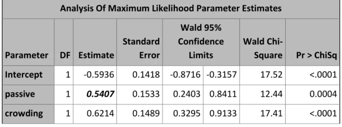
Table 8a. Poisson regression model of counts of LRI events adjusted for effect of passive smoking which was adjusted for crowding

Analysis Of Maximum Likelihood Parameter Estimates

Parameter DF Estimate

Standard Error

Wald 95% Confidence

Limits

Wald

Chi-Square Pr > ChiSq

Intercept 1 -0.5936 0.1418 -0.8716 -0.3157 17.52 <.0001 passive 1 0.5407 0.1533 0.2403 0.8411 12.44 0.0004 crowding 1 0.6214 0.1489 0.3295 0.9133 17.41 <.0001

Table 8b. Negative binomial regression model of counts of LRI events adjusted for effect of passive smoking which was adjusted for crowding

Analysis Of Maximum Likelihood Parameter Estimates

Parameter DF Estimate

Standard Error

Wald 0.95onfidence

Limits

Wald

Chi-Square Pr > ChiSq

Intercept 1 -0.562 0.176 -0.907 -0.216 10.15 0.0014 passive 1 0.570 0.200 0.178 0.963 8.10 0.0044 crowding 1 0.608 0.197 0.223 0.994 9.55 0.0020 Dispersion 1 1.035 0.268 0.623 1.718

Table 9a. Poisson regression model of counts of LRI events adjusted for effect of passive smoking where crowding is not present (i.e. crowding=0)

Analysis Of Maximum Likelihood Parameter Estimates

Parameter DF Estimate

Standard Error

Wald 95% Confidence

Limits

Wald

Chi-Square Pr > ChiSq

Zhou 15

Table 9b. Negative binomial regression model of counts of LRI events adjusted for effect of passive smoking where crowding is not present (i.e. crowding=0)

Analysis Of Maximum Likelihood Parameter Estimates

Parameter DF Estimate

Standard Error

Wald 95% Confidence Limits

Wald

Chi-Square Pr > ChiSq

Intercept 1 -0.581 0.230 -1.031 -0.132 6.42 0.0113 passive 1 0.656 0.324 0.022 1.290 4.11 0.0427 Dispersion 1 1.864 0.634 0.957 3.631

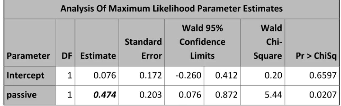
Table 10a. Poisson regression model of counts of LRI events adjusted for effect of passive smoking where crowding is present (i.e. crowding=1)

Analysis Of Maximum Likelihood Parameter Estimates

Parameter DF Estimate

Standard

Error

Wald 95% Confidence

Limits

Wald

Chi-Square Pr > ChiSq

Intercept 1 0.076 0.172 -0.260 0.412 0.20 0.6597 passive 1 0.474 _{0.203 0.076 0.872 5.44 0.0207}

Table 10b. Negative binomial regression model of counts of LRI events adjusted for effect of passive smoking where crowding is present (i.e. crowding=1)

Analysis Of Maximum Likelihood Parameter Estimates

Parameter DF Estimate

Standard Error

Wald 95% Confidence

Limits

Wald

Chi-Square Pr > ChiSq

Zhou 16

Table 11a. Poisson regression model of counts of LRI events adjusted for effect of passive smoking

Analysis Of Maximum Likelihood Parameter Estimates

Parameter DF Estimate

Standard Error

Wald 95% Confidence

Limits

Wald

Chi-Square Pr > ChiSq

Intercept 1 -0.340 0.122 -0.580 -0.101 7.76 0.0054 passive 1 0.658 0.150 0.362 0.953 19.02 <.0001

Table 11b. Negative binomial regression model of counts of LRI events adjusted for effect of passive smoking

Analysis Of Maximum Likelihood Parameter Estimates

Parameter DF Estimate

Standard Error

Wald 95% Confidence

Limits

Wald

Chi-Square Pr > ChiSq

Intercept 1 -0.302 0.156 -0.608 0.004 3.75 0.0527 passive 1 0.680 0.202 0.284 1.075 11.32 0.0008 Dispersion 1 1.194 0.288 0.745 1.914

Density Ratio Method

The incidence density ratio method described in LaVange et al. (1994) was used to

determine the density ratios for the four different outcomes. The average count (6) and average

time at-risk (c̅) were determined through PROC MEANS in SAS to produce an estimate of R for each model by exposure to passive smoking and no exposure to passive smoking. The variable

f =(QN ib_b̅ N) was computed, and the relationship between the variance of logm and the variance

of f was calculated to determine the 95% confidence intervals for

λ

calculated by _mb<|m’/_S<Smb<|m’. The 95% confidence intervals for the incidence density

ratios were calculated by

Zhou 17

Table 12 summarizes the results obtained from the density ratio method and the model-based

methods. All results in Table 12 have been converted from the natural log (loge) scale.

Table 12. Comparison between results from density ratio method and model-based methods (Poisson regression and Negative binomial regression)

Method Effect of passive

smoking, adjusted for crowding Effect of Passive smoking Effect of Passive smoking, where crowding = 0

Effect of Passive

smoking, where crowding = 1 Density Ratio Estimate 95%CI p-value 1.70 (1.17, 2.47) 0.0054 1.93 (1.33, 2.81) 0.0006 1.87 (1.01, 3.44) 0.0454 1.61 (1.00, 2.58) 0.0496 Poisson (unadjusted)

Estimate 95%CI p-value 1.72 (1.27, 2.32) <0.0001 1.93 (1.44, 2.59) < 0.0001 1.87 (1.19, 2.93) 0.0063 1.61 (1.08, 2.39) 0.0163 Negative Binomial Estimate 95%CI p-value 1.77 (1.19, 2.62) 0.0046 1.97 (1.33, 2.93) 0.0008 1.93 (1.02, 3.63) 0.0438 1.64 ( 0.99, 2.71)

0.0545

Discussion

This thesis evaluated different statistical methods for comparing counts of events for

at-risk time periods across two groups, such as the Wilcoxon rank sum test, Poisson regression,

negative binomial regression, and the density ratio method. The bleeding frequency dataset

(Nichols 2013) was used to evaluate the first three methods. The primary outcome of interest was

the rate of bleeds per year (over total follow-up time) and the secondary outcome of interest was

the frequency of bleeds in the first year. The mean and the standard deviations of the mean

bleeds for both outcome variables suggested that tolerized treatment reduced the frequency of

bleeds in dogs with hemophilia B. Due to the small sample size of the bleeding frequency dataset,

applying the Wilcoxon rank sum test was of particular interest to test the inference suggested by

the means and standard deviations, because it does not have any underlying distribution

assumptions. For both outcome variables, the Wilcoxon rank sum test had a significant two-sided

p-value (0.0003 and 0.0060, respectively). Thus, there is sufficient evidence to suggest that there

Zhou 18

dogs for both outcomes. The Somer’s D, Mann-Whitney estimator, and Hodges-Lehmann

confidence interval were also in agreement with the Wilcoxon rank sum test results. For both

outcome variables, Somer’s D was close to -1, the Mann-Whitney estimator was close to 0, and

the Hodges-Lehmann confidence interval did not contain 0, indicating the comparisons between

randomly selected subjects in the non-tolerized group and randomly selected subjects in the

tolerized group strongly favor the tolerized group. In other words, the dogs in the non-tolerized

group had a higher likelihood of having more bleeds than dogs in the tolerized group. This

supports the notion the tolerized treatment reduces the likelihood of having a bleed in hemophilia

B dogs.

Generally, when data are in the form of counts over a period of time at-risk, the

model-based method of Poisson regression is used because it is easily applied to this type of data.

However, the Poisson regression model assumes that there is a common rate for all subjects, and

thus it will under-estimate the variance of the parameter if this assumption is not met. To correct

for over-dispersion in the bleeding frequency dataset (Nichols 2013), scaled Poisson regression

and negative binomial regression were applied.

These three model-based methods produce similar models. As expected, the Poisson

regression model incorrectly had the narrowest 95% confidence interval since over-dispersion

was a factor in the bleeding frequency dataset. The 95% confidence interval for the negative

binomial regression model was narrower than the scaled Poisson regression model for both

outcome variables (respectively, (0.10, 0.84) versus (0.12, 0.64) for frequency of bleeds in first

year, and (0.09, 0.82) versus (0.12, 0.56) for rate of bleeds per year over two years of follow-up).

This indicates that the scaled Poisson model, which intended to correct for dispersion,

over-estimated the variance. Consequently, the negative binomial regression model is a more

appealing option than other corrections because it corrects for over-dispersion in a Poisson

regression with a better model. However, since it still assumes that each subject has an

underlying conditional Poisson distribution, it is not appropriate to use in the case of a small

sample size (less than or equal to 10 subjects per group) or any time that assumption is not met.

Sample size for a future study based on the results of a Wilcoxon rank sum test and a

negative binomial regression were calculated. Assuming that there will be an equal number of

subjects in the two groups and 0.90 power is desired, the sample size via the negative binomial

Zhou 19

size via the Wilcoxon rank sum method was approximately 11 subjects per group. Since the

sample size approximation assumed the continuity correction was about 0, the adjusted sample

size per group to achieve the desired power produced a sample size of 12 subjects per group.

The sample sizes calculated from both methods agree with each other.

The density ratio method provides an additional method that, like the Wilcoxon rank sum

method, has minimal assumptions for the underlying distributions. Furthermore, it provides a

direct way to analyze disease incidence. Unfortunately, the density ratio method requires large

sample size; therefore, it is not applicable to the bleeding frequency dataset. Instead, the dataset

of lower respiratory incidence (LRI) in infants during their first year from LaVange et al. (1994)

was used. The main effect of interest was passive smoking adjusted for crowding, though the

effect of passive smoking on LRI and the effect of passive smoking by crowding status (i.e., the

presence of crowding and no crowding) were also analyzed.

Poisson regression and negative binomial regression were also applied as model-based

methods. Over-dispersion was present in the LRI dataset, and thus negative binomial regression

was more appropriate than Poisson regression. As expected, for all four models, the 95%

confidence interval from Poisson regression was inappropriately narrower than from the negative

binomial model. The estimated standard errors for the parameters in all models were higher in

the negative binomial regression than in Poisson regression.

When the density ratio method was applied to estimate the four effects, the estimates

were more similar to the Poisson regression models. However, the 95% confidence intervals

were wider than the Poisson models. Instead, they were more similar to the negative binomial 95%

confidence intervals. A narrower 95% confidence interval than the negative binomial regression

model indicates that the density ratio method adequately adjusts for the over-dispersion, but is a

more precise method than negative binomial regression.

From these statistical considerations of different methods that deal with data of counts

over a time at-risk, it can be concluded that even though Poisson regression is most readily

applied to this type of data, it may not be the most appropriate model. When its distributional

assumptions are not met, Poisson regressions will inappropriately under-estimates the variance.

In the case of over-dispersion, the correction scaled Poisson regression may over-correct and

thus over-estimate the variance. Negative binomial regression provides a more appealing method

Zhou 20

However, in datasets where the assumption that every subject has an underlying Poisson

regression is not met, the negative binomial model is also not the most appropriate method.

In cases where assumptions about the underlying distribution are not met, the

non-parametric Wilcoxon rank sum test and alternative density ratio method are more appropriate to

apply than the model-based methods mentioned above. When the sample size is small, the

non-parametric Wilcoxon rank sum test is most commonly used. However, the power of a Wilcoxon

rank sum test can be adversely affected by other differences, such as shape and scale, instead of

just location. Furthermore, measures of differences for groups, such as Hodges-Lehmann and

Mann-Whitney estimators, may not be straightforward to obtain or interpret. The density ratio

method, on the other hand, cannot be used with small datasets and it is not as flexible in regard to

the number and types of covariates allowed in the model. However, with large sample sizes, the

density ratio method provides a direct method to evaluate incidence densities and produces more

precise estimates than the model-based methods. These considerations and other aspects are

important to evaluate because it will inform use of the most appropriate method to produce valid

estimates and inferences from the data.

References

LaVange L., Keyes L., Koch G., and Margolis P. Application of Sample Survey Methods for

Modelling Ratios to incidence Densities. Statistics in Medicine, 1994; 13: 343-355.

LaVange L., and Koch G. Rank Score Tests. Circulation, 2006; 114(23):2528-33.

Kappos L., Antel J., Comi G., Montalban X., O’Connor P., Polman C., Haas T., Korn A.,

Karlsson G., and Radue E., Oral Fingolimod (FTY720) for Relapsing Multiple Sclerosis.

The New England Journal of Medicine, 2006; 355: 1124-1140

Keene O., Jones M., Lane P., and Anderson J. Analysis of exacerbation rates in asthma and

chronic obstructive pulmonary disease: example from TRISTAN study. Pharmaceutical

Statistics, 2007; 6: 89-97.

Keene O., Calverley P., Jones P., Vesbo J., and Anderson J. Statistical analysis of exacerbation

rates in COPD: TRISTAN and ISOLDE revisited. European Respiratory Journal, 2008;

Zhou 21

Koch G. and Stokes M. Stokes. Some Nonparametric and Regression Model Strategies for

Counts of Primary Events from Randomized Studies. International Journal of Statistical

Sciences, 2006; 5

Kotz-Johnson. Poisson Regression. Encyclopedia of Statistical Sciences, 1986; 7

Nichols T., Bellinger D., and Raymer R. Version 4: Effect of AAV8-mediated expression of

canine FVIIa on bleeding frequency of hemophilia A dogs. 2013

Saville B., LaVange L., and Koch G. Estimating Covariate-Adjusted Incidence Density Ratios

for Multiple Time Intervals in Clinical Trials Using Nonparametric Randomization-based

ANCOVA. Statistics in Biopharmaceutical Research, 2011; 3 (2).

Stokes M., Davis C., and Koch G. Categorical Data Analysis Using SAS Third Edition. : 2012,

Chapter 5, 12, 15.

Appendix 1: Sample Size via Wilcoxon rank sum method

We will use a transformation of the power definition to calculate the needed sample size. The

following calculations are for the normal approximation of the Wilcoxon rank sum test.

For the Wilcoxon rank sum test, _i = ( − ) is the difference between mean ranks for group 1 and group 2.

The null hypothesis, H0, is the distributions for Group 1 and Group 2 are equal. Let ž = ( + ), then

*{( − )|;  } = 0 and

-.{( − )|;  , 9 4357} = ¡_n1 +

1 n£

∑ (Y − (ž + 1) 2) ⁄

]T

(ž − 1)

= (=)

S%S!

If = n = ¦

§ , then Var{( − )|;  } ==> .

We know that ¨¦ ©

S%S!§ − 0.5ª = i% i!

, where ©

S%S! is the Mann-Whitney Statistic.

If = =

, then -. ¨¦ ©

S%S!§ «; ª = = >!

The alternative hypothesis, HA, is that the two distributions are not equal. In other words,

HA: * ¨¦ ©

Zhou 22 ­9®5. = (1 −

β

(°%°!)

" %!¦›%%=›!%§

#"$%_&"! > A±;²³, where (S%+

S!) is the continuity

correction.

If = =

, then ­9®5. = 1 −

β

(. ) !_"! #("$%)/&"!·;²(

is cumulative density function of N(0,1), then

1 − = (. ) !"!

#"$%_&"! − A/(

where ) = *{Mann-Whitney estimator} and ¦

!§ is the continuity correction.

@A/+ DE¡ž + 1_3ž £ = »() − 0.5) −_ž2¼

Since ž + 1

≅

!) ≅ 0, @A/+ DE¦_> § = () − 0.5)

N= + =

½Z' !=Z[¾

!

>(µ  .¿)!

= =½Z

' !=Z[¾

!

À(µ  .¿)!

To determine a sample size needed for 0.90 power at two-sided V = 0.05, Zα/2 = 1.96, Zβ = 1.282.

The power for a given calculated sample size N can be verified with (1). It is expected that the

power calculated with calculated N will be less than the power desired so one subject per group

is added.

Appendix 2: Poisson Regression and Negative Binomial Regression

Subjects are assumed to represent a population comparable, in a sense, to a random sample. Let 6 denote the count of events and 4 denote time at-risk.

Let Y = 1,2 denote two groups of subjects and 3 = 1,2, … , denote subjects in the kth group.

Poisson regression:

For 3 = 1,2, … , let 6 be the count of events for subject 3 and 4 be the exposure (time at-risk)

for subject 3

Zhou 23

Poisson regression assumes that each subject’s respective 6 has an independent Poisson distribution. Thus,

E(6)=Var(6) = μ =

λ

The likelihood function is ∏ exp (−λ4)(”NON)PN QN! S

T .

The usual model for the

λ

λ

explanatory variables and β as the vector of unknown parameters. β is estimated by the

maximum likelihood.

When

λ

λ

λ

Ä , thus

-.@

λ

λ

Æ §

=Ç È

λ

Ä É

= ∑ 6/(∑ 4) = q_λÅ

Negative Binomial:

A negative binomial model combines Poisson regression with a model error that follows a

gamma distribution.

For 3 = 1,2, … , , 6 has the Poisson distribution with a givenλ_Ê and t_Ê, where 4 is the fixed

duration of follow-up and U has gamma distribution with parameters (V, W). Thus,

E(6)= U4, Furthermore,

E(U)= VW and Var(U) = VW .

The usual model for negative binomial regression is exp(X) = c′ ∗ with offset log_m(4),

where c’ is the vector of explanatory variables and β is the vector of unknown parameters

estimated by maximum likelihood.

Assume V = V for all patients, then U has density function

Ï(U )=

λ

ÓN ÔN£

Zhou 24 Then,

*(6|U) = U4 and *(6) = *@*(6|U)E

= *(U4)

= VWt_Ê= μ. and

Var(yÊ) = -.{*(6|U)} + *{-.(6|U)}

= -.{U4} + *{U4}

= αW4+αW4

= N! α + X = X + YX,

where Y is the negative binomial dispersion factor.

For fixed U, as α gets large (or as Y approaches 0), the negative binomial distribution converges