Quality
United States
Environmental Protection Agency
Guidance for
Data Quality Assessment
Practical Methods for
Data Analysis
EPA QA/G-9
QA00 UPDATE
Office of Environmental InformationWashington, DC 20460
EPA/600/R-96/084 July, 2000
EPA QA/G-9 Final
QA00 Version i July 2000
FOREWORD
This document is the 2000 (QA00) version of the Guidance for Data Quality Assessment which provides general guidance to organizations on assessing data quality criteria and
performance specifications for decision making. The Environmental Protection Agency (EPA) has developed a process for performing Data Quality Assessment (DQA) Process for project
managers and planners to determine whether the type, quantity, and quality of data needed to support Agency decisions has been achieved. This guidance is the culmination of experiences in the design and statistical analyses of environmental data in different Program Offices at the EPA. Many elements of prior guidance, statistics, and scientific planning have been incorporated into this document.
This document is distinctly different from other guidance documents; it is not intended to be read in a linear or continuous fashion. The intent of the document is for it to be used as a "tool-box" of useful techniques in assessing the quality of data. The overall structure of the document will enable the analyst to investigate many different problems using a systematic methodology.
This document is one of a series of quality management guidance documents that the EPA Quality Staff has prepared to assist users in implementing the Agency-wide Quality System. Other related documents include:
EPA QA/G-4 Guidance for the Data Quality Objectives Process
EPA QA/G-4D DEFT Software for the Data Quality Objectives Process
EPA QA/G-4HW Guidance for the Data Quality Objectives Process for Hazardous
Waste Site Investigations
EPA QA/G-9D Data Quality Evaluation Statistical Toolbox (DataQUEST)
This document is intended to be a "living document" that will be updated periodically to incorporate new topics and revisions or refinements to existing procedures. Comments received on this 2000 version will be considered for inclusion in subsequent versions. Please send your written comments on Guidance for Data Quality Assessment to:
Quality Staff (2811R)
Office of Environmental Information U.S. Environmental Protection Agency 1200 Pennsylvania Avenue, NW Washington, DC 20460
Phone: (202) 564-6830 Fax: (202) 565-2441 E-mail: [email protected]
EPA QA/G-9 Final
QA00 Version iii July 2000
TABLE OF CONTENTS
Page INTRODUCTION . . . 0 - 1
0.1 PURPOSE AND OVERVIEW . . . 0 - 1 0.2 DQA AND THE DATA LIFE CYCLE . . . 0 - 2 0.3 THE 5 STEPS OF DQA . . . 0 - 2 0.4 INTENDED AUDIENCE . . . 0 - 4 0.5 ORGANIZATION . . . 0 - 4 0.6 SUPPLEMENTAL SOURCES . . . 0 - 4
STEP 1: REVIEW DQOs AND THE SAMPLING DESIGN . . . 1 - 1
1.1 OVERVIEW AND ACTIVITIES . . . 1 - 3 1.1.1 Review Study Objectives . . . 1 - 4 1.1.2 Translate Objectives into Statistical Hypotheses . . . 1 - 4 1.1.3 Develop Limits on Decision Errors . . . 1 - 5 1.1.4 Review Sampling Design . . . 1 - 7
1.2 DEVELOPING THE STATEMENT OF HYPOTHESES . . . 1 - 9
1.3 DESIGNS FOR SAMPLING ENVIRONMENTAL MEDIA . . . 1 - 11
1.3.1 Authoritative Sampling . . . 1 - 11 1.3.2 Probability Sampling . . . 1 - 13 1.3.2.1 Simple Random Sampling . . . 1 - 13 1.3.2.2 Sequential Random Sampling . . . 1 - 13 1.3.2.3 Systematic Samples . . . 1 - 14 1.3.2.4 Stratified Samples . . . 1 - 14 1.3.2.5 Compositing Physical Samples . . . 1 - 15 1.3.2.6 Other Sampling Designs . . . 1 - 15
STEP 2: CONDUCT A PRELIMINARY DATA REVIEW . . . 2 - 1
2.1 OVERVIEW AND ACTIVITIES . . . 2 - 3 2.1.1 Review Quality Assurance Reports . . . 2 - 3 2.1.2 Calculate Basic Statistical Quantities . . . 2 - 4 2.1.3 Graph the Data . . . 2 - 4 2.2 STATISTICAL QUANTITIES . . . 2 - 5 2.2.1 Measures of Relative Standing . . . 2 - 5 2.2.2 Measures of Central Tendency . . . 2 - 6 2.2.3 Measures of Dispersion . . . 2 - 8 2.2.4 Measures of Association . . . 2 - 8 2.2.4.1 Pearson’s Correlation Coefficient . . . 2 - 8 2.2.4.2 Spearman’s Rank Correlation Coefficient . . . 2 - 11 2.2.4.3 Serial Correlation Coefficient . . . 2 - 11
Page
2.3 GRAPHICAL REPRESENTATIONS . . . 2 - 13 2.3.1 Histogram/Frequency Plots . . . 2 - 13 2.3.2 Stem-and-Leaf Plot . . . 2 - 15 2.3.3 Box and Whisker Plot . . . 2 - 17 2.3.4 Ranked Data Plot . . . 2 - 17 2.3.5 Quantile Plot . . . 2 - 21 2.3.6 Normal Probability Plot (Quantile-Quantile Plot) . . . 2 - 22 2.3.7 Plots for Two or More Variables . . . 2 - 26 2.3.7.1 Plots for Individual Data Points . . . 2 - 26 2.3.7.2 Scatter Plot . . . 2 - 27 2.3.7.3 Extensions of the Scatter Plot . . . 2 - 27 2.3.7.4 Empirical Quantile-Quantile Plot . . . 2 - 30 2.3.8 Plots for Temporal Data . . . 2 - 30 2.3.8.1 Time Plot . . . 2 - 32 2.3.8.2 Plot of the Autocorrelation Function (Correlogram) . . . 2 - 33 2.3.8.3 Multiple Observations Per Time Period . . . 2 - 35 2.3.9 Plots for Spatial Data . . . 2 - 36 2.3.9.1 Posting Plots . . . 2 - 37 2.3.9.2 Symbol Plots . . . 2 - 37 2.3.9.3 Other Spatial Graphical Representations . . . 2 - 39 2.4 Probability Distributions . . . 2 - 39 2.4.1 The Normal Distribution . . . 2 - 39 2.4.2 The t-Distribution . . . 2 - 40 2.4.3 The Lognormal Distribution . . . 2 - 40 2.4.4 Central Limit Theorem . . . 2 - 41
STEP 3: SELECT THE STATISTICAL TEST . . . 3 - 1
3.1 OVERVIEW AND ACTIVITIES . . . 3 - 3 3.1.1 Select Statistical Hypothesis Test . . . 3 - 3 3.1.2 Identify Assumptions Underlying the Statistical Test . . . 3 - 3
3.2 TESTS OF HYPOTHESES ABOUT A SINGLE POPULATION . . . 3 - 4
3.2.1 Tests for a Mean . . . 3 - 4 3.2.1.1 The One-Sample t-Test . . . 3 - 5 3.2.1.2 The Wilcoxon Signed Rank (One-Sample) Test . . . 3 - 11 3.2.1.3 The Chen Test . . . 3 - 15 3.2.2 Tests for a Proportion or Percentile . . . 3 - 16 3.2.2.1 The One-Sample Proportion Test . . . 3 - 18 3.2.3 Tests for a Median . . . 3 - 18 3.2.4 Confidence Intervals . . . 3 - 20 3.3 TESTS FOR COMPARING TWO POPULATIONS . . . 3 - 21
EPA QA/G-9 Final
QA00 Version v July 2000
Page
3.3.1 Comparing Two Means . . . 3 - 22 3.3.1.1 Student's Two-Sample t-Test (Equal Variances) . . . 3 - 23 3.3.1.2 Satterthwaite's Two-Sample t-Test (Unequal Variances) . . 3 - 23 3.3.2 Comparing Two Proportions or Percentiles . . . 3 - 27 3.3.2.1 Two-Sample Test for Proportions . . . 3 - 28 3.3.3 Nonparametric Comparisons of Two Population . . . 3 - 31 3.3.3.1 The Wilcoxon Rank Sum Test . . . 3 - 31 3.3.3.2 The Quantile Test . . . 3 - 35 3.3.4 Comparing Two Medians . . . 3 - 36 3.4 Tests for Comparing Several Populations . . . 3 - 37 3.4.1 Tests for Comparing Several Means . . . 3 - 37 3.4.1.1 Dunnett’s Test . . . 3 - 38
STEP 4: VERIFY THE ASSUMPTIONS OF THE STATISTICAL TEST . . . 4 - 1
4.1 OVERVIEW AND ACTIVITIES . . . 4 - 3 4.1.1 Determine Approach for Verifying Assumptions . . . 4 - 3 4.1.2 Perform Tests of Assumptions . . . 4 - 4 4.1.3 Determine Corrective Actions . . . 4 - 5 4.2 TESTS FOR DISTRIBUTIONAL ASSUMPTIONS . . . 4 - 5 4.2.1 Graphical Methods . . . 4 - 7 4.2.2 Shapiro-Wilk Test for Normality (the W test) . . . 4 - 8 4.2.3 Extensions of the Shapiro-Wilk Test (Filliben's Statistic) . . . 4 - 8 4.2.4 Coefficient of Variation . . . 4 - 8 4.2.5 Coefficient of Skewness/Coefficient of Kurtosis Tests . . . 4 - 9 4.2.6 Range Tests . . . 4 - 10 4.2.7 Goodness-of-Fit Tests . . . 4 - 12 4.2.8 Recommendations . . . 4 - 13 4.3 TESTS FOR TRENDS . . . 4 - 13 4.3.1 Introduction . . . 4 - 13 4.3.2 Regression-Based Methods for Estimating and Testing for Trends . 4 - 14 4.3.2.1 Estimating a Trend Using the Slope of the Regression Line 4 - 14 4.3.2.2 Testing for Trends Using Regression Methods . . . 4 - 15 4.3.3 General Trend Estimation Methods . . . 4 - 16 4.3.3.1 Sen's Slope Estimator . . . 4 - 16 4.3.3.2 Seasonal Kendall Slope Estimator . . . 4 - 16 4.3.4 Hypothesis Tests for Detecting Trends . . . 4 - 16
4.3.4.1 One Observation per Time Period for
One Sampling Location . . . 4 - 16 4.3.4.2 Multiple Observations per Time Period
Page
4.3.4.3 Multiple Sampling Locations with Multiple Observations . 4 - 20 4.3.4.4 One Observation for One Station with Multiple Seasons . 4 - 22 4.3.5 A Discussion on Tests for Trends . . . 4 - 23 4.3.6 Testing for Trends in Sequences of Data . . . 4 - 24 4.4 OUTLIERS . . . 4 - 24 4.4.1 Background . . . 4 - 24 4.4.2 Selection of a Statistical Test . . . 4 - 27 4.4.3 Extreme Value Test (Dixon's Test) . . . 4 - 27 4.4.4 Discordance Test . . . 4 - 29 4.4.5 Rosner's Test . . . 4 - 30 4.4.6 Walsh's Test . . . 4 - 32 4.4.7 Multivariate Outliers . . . 4 - 32 4.5 TESTS FOR DISPERSIONS . . . 4 - 33 4.5.1 Confidence Intervals for a Single Variance . . . 4 - 33 4.5.2 The F-Test for the Equality of Two Variances . . . 4 - 33 4.5.3 Bartlett's Test for the Equality of Two or More Variances . . . 4 - 33 4.5.4 Levene's Test for the Equality of Two or More Variances . . . 4 - 35 4.6 TRANSFORMATIONS . . . 4 - 39 4.6.1 Types of Data Transformations . . . 4 - 39 4.6.2 Reasons for Transforming Data . . . 4 - 41 4.7 VALUES BELOW DETECTION LIMITS . . . 4 - 42 4.7.1 Less than 15% Nondetects - Substitution Methods . . . 4 - 43 4.7.2 Between 15-50% Nondetects . . . 4 - 43 4.7.2.1 Cohen's Method . . . 4 - 43 4.7.2.2 Trimmed Mean . . . 4 - 45 4.7.2.3 Winsorized Mean and Standard Deviation . . . 4 - 45 4.7.2.4 Atchison’s Method . . . 4 - 46 4.7.2.5 Selecting Between Atchison’s Method or Cohen’s Method . 4 - 49 4.7.3 Greater than 5-% Nondetects - Test of Proportions . . . 4 - 50 4.7.4 Recommendations . . . 4 - 50 4.8 INDEPENDENCE . . . 4 - 51
STEP 5: DRAW CONCLUSIONS FROM THE DATA . . . 5 - 1
5.1 OVERVIEW AND ACTIVITIES . . . 5 - 3 5.1.1 Perform the Statistical Hypothesis Test . . . 5 - 3 5.1.2 Draw Study Conclusions . . . 5 - 3 5.1.3 Evaluate Performance of the Sampling Design . . . 5 - 5
5.2 INTERPRETING AND COMMUNICATING THE TEST RESULTS . . . 5 - 6
5.2.1 Interpretation of p-Values . . . 5 - 7 5.2.2 "Accepting" vs. "Failing to Reject" the Null Hypothesis . . . 5 - 7
EPA QA/G-9 Final
QA00 Version vii July 2000
Page
5.2.3 Statistical Significance vs. Practical Significance . . . 5 - 8 5.2.4 Impact of Bias on Test Results . . . 5 - 8 5.2.5 Quantity vs. Quality of Data . . . 5 - 11 5.2.6 "Proof of Safety" vs. "Proof of Hazard" . . . 5 - 12
APPENDIX A: STATISTICAL TABLES . . . A - 1 APPENDIX B: REFERENCES . . . B - 2
EPA QA/G-9 Final
QA00 Version 0 - 1 July 2000
INTRODUCTION
0.1 PURPOSE AND OVERVIEW
Data Quality Assessment (DQA) is the scientific and statistical evaluation of data to determine if data obtained from environmental data operations are of the right type, quality, and quantity to support their intended use. This guidance demonstrates how to use DQA in
evaluating environmental data sets and illustrates how to apply some graphical and statistical tools for performing DQA. The guidance focuses primarily on using DQA in environmental decision making; however, the tools presented for preliminary data review and verifying statistical
assumptions are useful whenever environmental data are used, regardless of whether the data are used for decision making.
DQA is built on a fundamental premise: data quality, as a concept, is meaningful only when it relates to the intended use of the data. Data quality does not exist in a vacuum; one must know in what context a data set is to be used in order to establish a relevant yardstick for judging whether or not the data set is adequate. By using the DQA, one can answer two fundamental questions:
1. Can the decision (or estimate) be made with the desired confidence, given the quality of the data set?
2. How well can the sampling design be expected to perform over a wide range of possible outcomes? If the same sampling design strategy is used again for a similar study, would the data be expected to support the same intended use with the desired level of
confidence, particularly if the measurement results turned out to be higher or lower than those observed in the current study?
The first question addresses the data user's immediate needs. For example, if the data provide evidence strongly in favor of one course of action over another, then the decision maker can proceed knowing that the decision will be supported by unambiguous data. If, however, the data do not show sufficiently strong evidence to favor one alternative, then the data analysis alerts the decision maker to this uncertainty. The decision maker now is in a position to make an
informed choice about how to proceed (such as collect more or different data before making the decision, or proceed with the decision despite the relatively high, but acceptable, probability of drawing an erroneous conclusion).
The second question addresses the data user's potential future needs. For example, if investigators decide to use a certain sampling design at a different location from where the design was first used, they should determine how well the design can be expected to perform given that the outcomes and environmental conditions of this sampling event will be different from those of the original event. Because environmental conditions will vary from one location or time to another, the adequacy of the sampling design approach should be evaluated over a broad range of possible outcomes and conditions.
IMPLEMENTATION
Field Data Collection and Associated Quality Assurance / Quality Control Activities
PLANNING
Data Quality Objectives Process Quality Assurance Project Plan Development
ASSESSMENT
Data Validation/Verification Data Quality Assessment
OUTPUT
INPUT
OUTPUT QUALITY ASSURANCE ASSESSMENT
CONCLUSIONS DRAWN FROM DATA DATA VALIDATION/VERIFICATION
Verify measurement performance Verify measurement procedures and reporting requirements
VALIDATED/VERIFIED DATA
DATA QUALITY ASSESSMENT Review DQOs and design Conduct preliminary data review Select statistical test
Verify assumptions Draw conclusions
QC/Performance Evaluation Data Routine Data
INPUTS
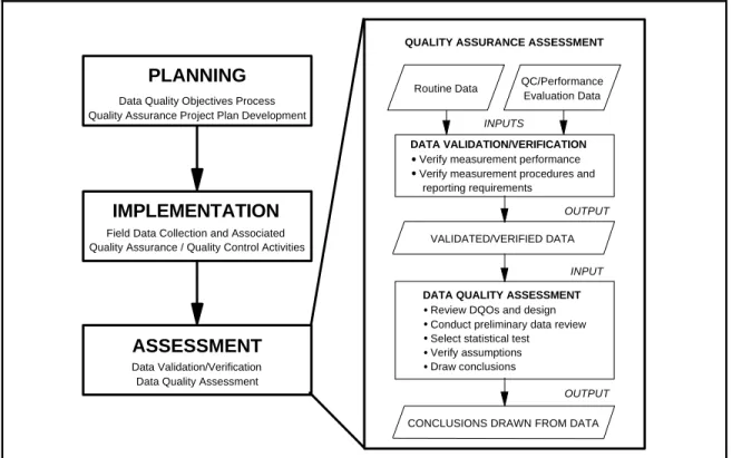
Figure 0-1. DQA in the Context of the Data Life Cycle
0.2 DQA AND THE DATA LIFE CYCLE
The data life cycle (depicted in Figure 0-1) comprises three steps: planning,
implementation, and assessment. During the planning phase, the Data Quality Objectives (DQO) Process (or some other systematic planning procedure) is used to define quantitative and
qualitative criteria for determining when, where, and how many samples (measurements) to collect and a desired level of confidence. This information, along with the sampling methods, analytical procedures, and appropriate quality assurance (QA) and quality control (QC)
procedures, are documented in the QA Project Plan. Data are then collected following the QA Project Plan specifications. DQA completes the data life cycle by providing the assessment needed to determine if the planning objectives were achieved. During the assessment phase, the data are validated and verified to ensure that the sampling and analysis protocols specified in the QA Project Plan were followed, and that the measurement systems performed in accordance with the criteria specified in the QA Project Plan. DQA then proceeds using the validated data set to determine if the quality of the data is satisfactory.
0.3 THE 5 STEPS OF THE DQA
The DQA involves five steps that begin with a review of the planning documentation and end with an answer to the question posed during the planning phase of the study. These steps roughly parallel the actions of an environmental statistician when analyzing a set of data. The five
EPA QA/G-9 Final
QA00 Version 0 - 3 July 2000
steps, which are described in detail in the remaining chapters of this guidance, are briefly summarized as follows:
1. Review the Data Quality Objectives (DQOs) and Sampling Design: Review the DQO outputs to assure that they are still applicable. If DQOs have not been developed, specify DQOs before evaluating the data (e.g., for environmental decisions, define the statistical hypothesis and specify tolerable limits on decision errors; for estimation problems, define an acceptable confidence or probability interval width). Review the sampling design and data collection documentation for consistency with the DQOs.
2. Conduct a Preliminary Data Review: Review QA reports, calculate basic statistics, and generate graphs of the data. Use this information to learn about the structure of the data and identify patterns, relationships, or potential anomalies.
3. Select the Statistical Test: Select the most appropriate procedure for summarizing and analyzing the data, based on the review of the DQOs, the sampling design, and the preliminary data review. Identify the key underlying assumptions that must hold for the statistical procedures to be valid.
4. Verify the Assumptions of the Statistical Test: Evaluate whether the underlying assumptions hold, or whether departures are acceptable, given the actual data and other information about the study.
5. Draw Conclusions from the Data: Perform the calculations required for the statistical test and document the inferences drawn as a result of these calculations. If the design is to be used again, evaluate the performance of the sampling design.
These five steps are presented in a linear sequence, but the DQA is by its very nature iterative. For example, if the preliminary data review reveals patterns or anomalies in the data set that are inconsistent with the DQOs, then some aspects of the study planning may have to be reconsidered in Step 1. Likewise, if the underlying assumptions of the statistical test are not supported by the data, then previous steps of the DQA may have to be revisited. The strength of the DQA is that it is designed to promote an understanding of how well the data satisfy their intended use by
progressing in a logical and efficient manner.
Nevertheless, it should be emphasized that the DQA cannot absolutely prove that one has or has not achieved the DQOs set forth during the planning phase of a study. This situation occurs because a decision maker can never know the true value of the item of interest. Data collection only provides the investigators with an estimate of this, not its true value. Further, because analytical methods are not perfect, they too can only provide an estimate of the true value of an environmental sample. Because investigators make a decision based on estimated and not true values, they run the risk of making a wrong decision (decision error) about the item of interest.
0.4 INTENDED AUDIENCE
This guidance is written for a broad audience of potential data users, data analysts, and data generators. Data users (such as project managers, risk assessors, or principal investigators who are responsible for making decisions or producing estimates regarding environmental characteristics based on environmental data) should find this guidance useful for understanding and directing the technical work of others who produce and analyze data. Data analysts (such as quality assurance specialists, or any technical professional who is responsible for evaluating the quality of environmental data) should find this guidance to be a convenient compendium of basic assessment tools. Data generators (such as analytical chemists, field sampling specialists, or technical support staff responsible for collecting and analyzing environmental samples and reporting the resulting data values) should find this guidance useful for understanding how their work will be used and for providing a foundation for improving the efficiency and effectiveness of the data generation process.
0.5 ORGANIZATION
This guidance presents background information and statistical tools for performing DQA. Each chapter corresponds to a step in the DQA and begins with an overview of the activities to be performed for that step. Following the overviews in Chapters 1, 2, 3, and 4, specific graphical or statistical tools are described and step-by-step procedures are provided along with examples.
0.6 SUPPLEMENTAL SOURCES
Many of the graphical and statistical tools presented in this guidance are also implemented in a user-friendly, personal computer software program called Data Quality Evaluation Statistical Tools (DataQUEST) (G-9D) (EPA, 1996). DataQUEST simplifies the implementation of DQA by automating many of the recommended statistical tools. DataQUEST runs on most IBM-compatible personal computers using the DOS operating system; see the DataQUEST User's Guide for complete information on the minimum computer requirements.
EPA QA/G-9 Final
QA00 Version 1 - 1 July 2000
CHAPTER 1
STEP 1: REVIEW DQOs AND THE SAMPLING DESIGN
THE DATA QUALITY ASSESSMENT PROCESS
Review DQOs and Sampling Design
Conduct Preliminary Data Review
Select the Statistical Test
Verify the Assumptions
Draw Conclusions From the Data
REVIEW DQOs AND SAMPLING DESIGN
Purpose
Review the DQO outputs, the sampling design, and any data collection documentation for consistency. If DQOs have not been developed, define the statistical hypothesis and specify tolerable limits on decision errors.
Activities
Review Study Objectives
Translate Objectives into Statistical Hypothesis Develop Limits on Decision Errors
Review Sampling Design
Tools
Statements of hypotheses Sampling design concepts
! Review the objectives of the study.
P If DQOs have not been developed, review Section 1.1.1 and define these objectives.
P If DQOs were developed, review the outputs from the DQO Process.
! Translate the data user's objectives into a statement of the primary statistical hypothesis.
P If DQOs have not been developed, review Sections 1.1.2 and 1.2, and Box 1-1, then develop a statement of the hypothesis based on the data user's objectives.
P If DQOs were developed, translate them into a statement of the primary hypothesis.
! Translate the data user's objectives into limits on Type I or Type II decision errors.
P If DQOs have not been developed, review Section 1.1.3 and document the data user's tolerable limits on decision errors.
P If DQOs were developed, confirm the limits on decision errors.
! Review the sampling design and note any special features or potential problems.
P Review the sampling design for any deviations (Sections 1.1.4 and 1.3).
List of Boxes
Page Box 1-1: Example Applying the DQO Process Retrospectively . . . 1 - 8
List of Tables
Page Table 1-1. Choosing a Parameter of Interest . . . 1 - 6 Table 1-2. Commonly Used Statements of Statistical Hypotheses . . . 1 - 12
List of Figures
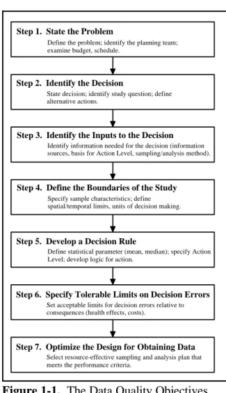
Page Figure 1-1. The Data Quality Objectives Process . . . 1 - 3
EPA QA/G-9 Final
QA00 Version 1 - 3 July 2000
Step 1. State the Problem
Define the problem; identify the planning team; examine budget, schedule.
Step 2. Identify the Decision
State decision; identify study question; define alternative actions.
Step 3. Identify the Inputs to the Decision Identify information needed for the decision (information sources, basis for Action Level, sampling/analysis method).
Step 4. Define the Boundaries of the Study Specify sample characteristics; define spatial/temporal limits, units of decision making.
Step 5. Develop a Decision Rule
Define statistical parameter (mean, median); specify Action Level; develop logic for action.
Step 6. Specify Tolerable Limits on Decision Errors Set acceptable limits for decision errors relative to consequences (health effects, costs).
Step 7. Optimize the Design for Obtaining Data Select resource-effective sampling and analysis plan that meets the performance criteria.
Figure 1-1. The Data Quality Objectives Process
CHAPTER 1
STEP 1: REVIEW DQOs AND THE SAMPLING DESIGN
1.1 OVERVIEW AND ACTIVITIES
DQA begins by reviewing the key outputs from the planning phase of the data life cycle: the Data Quality Objectives (DQOs), the Quality Assurance (QA) Project Plan, and any
associated documents. The DQOs provide the context for understanding the purpose of the data collection effort and establish the qualitative and quantitative criteria for assessing the quality of the data set for the intended use. The sampling design (documented in the QA Project Plan) provides important information about how to interpret the data. By studying the sampling design, the analyst can gain an understanding of the assumptions under which the design was developed, as well as the relationship between these assumptions and the DQOs. By reviewing the methods by which the samples were collected, measured, and reported, the analyst prepares for the preliminary data review and subsequent steps of DQA.
Careful planning improves the
representativeness and overall quality of a sampling design, the effectiveness and efficiency with which the sampling and analysis plan is implemented, and the usefulness of subsequent DQA efforts. Given the benefits of planning, the Agency has developed the DQO Process which is a logical, systematic planning procedure based on the scientific method. The DQO Process emphasizes the planning and development of a sampling design to collect the right type, quality, and quantity of data needed to support the decision. Using both the DQO Process and the DQA will help to ensure that the decisions are supported by data of adequate quality; the DQO Process does so prospectively and the DQA does so retrospectively.
When DQOs have not been developed during the planning phase of the study, it is necessary to develop statements of the data user's objectives prior to conducting DQA. The primary purpose of stating the data user's objectives prior to analyzing the data is to establish appropriate criteria for evaluating the quality of the data with respect to their intended use. Analysts who are not familiar with the DQO Process should refer to the Guidance for the Data Quality Objectives Process (QA/G-4) (1994), a book on statistical decision
1
Throughout this document, the term "primary hypotheses" refers to the statistical hypotheses that correspond to the data user's decision. Other statistical hypotheses can be formulated to formally test the assumptions that underlie the specific calculations used to test the primary hypotheses. See Chapter 3 for examples of assumptions underlying primary hypotheses and Chapter 4 for examples of how to test these underlying assumptions.
making using tests of hypothesis, or consult a statistician. The seven steps of the DQO Process are illustrated in Figure 1.1.
The remainder of this chapter addresses recommended activities for performing this step of DQA and technical considerations that support these activities. The remainder of this section describes the recommended activities, the first three of which will differ depending on whether DQOs have already been developed for the study. Section 1.2 describes how to select the null and alternative hypothesis and Section 1.3 presents a brief overview of different types of sampling designs.
1.1.1 Review Study Objectives
In this activity, the objectives of the study are reviewed to provide context for analyzing the data. If a planning process has been implemented before the data are collected, then this step reduces to reviewing the documentation on the study objectives. If no planning process was used, the data user should:
• Develop a concise definition of the problem (DQO Process Step 1) and the decision (DQO Process Step 2) for which the data were collected. This should provide the fundamental reason for collecting the environmental data and identify all potential actions that could result from the data analysis.
• Identify if any essential information is missing (DQO Process Step 3). If so, either collect the missing information before proceeding, or select a different approach to resolving the decision.
• Specify the scale of decision making (any subpopulations of interest) and any boundaries on the study (DQO Process Step 4) based on the sampling design. The scale of decision making is the smallest area or time period to which the decision will apply. The sampling design and implementation may restrict how small or how large this scale of decision making can be.
1.1.2 Translate Objectives into Statistical Hypotheses
In this activity, the data user's objectives are used to develop a precise statement of the primary1 hypotheses to be tested using environmental data. A statement of the primary statistical hypotheses includes a null hypothesis, which is a "baseline condition" that is presumed to be true in the absence of strong evidence to the contrary, and an alternative hypothesis, which bears the burden of proof. In other words, the baseline condition will be retained unless the alternative
EPA QA/G-9 Final
QA00 Version 1 - 5 July 2000
condition (the alternative hypothesis) is thought to be true due to the preponderance of evidence. In general, such hypotheses consist of the following elements:
• a population parameter of interest, which describes the feature of the environment that the data user is investigating;
• a numerical value to which the parameter will be compared, such as a regulatory or risk-based threshold or a similar parameter from another place (e.g., comparison to a reference site) or time (e.g., comparison to a prior time); and
• the relation (such as "is equal to" or "is greater than") that specifies precisely how the parameter will be compared to the numerical value.
To help the analyst decide what parameter value should be investigated, Table 1-1 compares the merits of the mean, upper proportion (percentile), and mean. If DQOs were developed, the statement of hypotheses already should be documented in the outputs of Step 6 of the DQO Process. If DQOs have not been developed, then the analyst should consult with the data user to develop hypotheses that address the data user's concerns. Section 1.2 describes in detail how to develop the statement of hypotheses and includes a list of common encountered hypotheses for environmental decisions.
1.1.3 Develop Limits on Decision Errors
The goal of this activity is to develop numerical probability limits that express the data user's tolerance for committing false rejection (Type I) or false acceptance (Type II) decision errors as a result of uncertainty in the data. A false rejection error occurs when the null hypothesis is rejected when it is true. A false acceptance decision error occurs when the null hypothesis is not rejected when it is false. These are the statistical definitions of false rejection and false acceptance decision errors. Other commonly used phrases include "level of significance" which is equal to the Type I Error (false rejection) and "complement of power" equal to the Type II Error (false acceptance). If tolerable decision error rates were not established prior to data collection, then the data user should:
• Specify the gray region where the consequences of a false acceptance decision error are relatively minor (DQO Process Step 6). The gray region is bounded on one side by the threshold value and on the other side by that parameter value where the consequences of making a false acceptance decision error begin to be significant. Establish this boundary by evaluating the consequences of not rejecting the null hypothesis when it is false and then place the edge of the gray region where these consequences are severe enough to set a limit on the magnitude of this false acceptance decision error. The gray region is the area between this parameter value and the threshold value.
The width of the gray region represents one important aspect of the decision maker's concern for decision errors. A more narrow gray region implies a desire to detect
Table 1-1. Choosing a Parameter of Interest
Parameter Points to Consider
Mean 1. Easy to calculate and estimate a confidence interval.
2. Useful when the standard has been based on consideration of health effects or long-term average exposure. 3. Useful when the data have little variation from sample to sample or season to season.
4. If the data have a large coefficient of variation (greater than about 1.5) testing the mean can require more samples than for testing an upper percentile in order to provide the same protection to human health and the environment.
5. Can have high false rejection rates with small sample sizes and highly skewed data, i.e., when the contamination levels are generally low with only occasional short periods of high contamination.
6. Not as powerful for testing attainment when there is a large proportion of less-than-detection-limit values. 7. Is adversely affected by outliers or errors in a few data values.
Upper Proportion (Percentile)
1. Requiring that an upper percentile be less than a standard can limit the occurrence of samples with high concentrations, depending on the selected percentile.
2. Unaffected by less-than-detection-limit values, as long as the detection limit is less than the cleanup standard.
3. If the health effects of the contaminant are acute, extreme concentrations are of concern and are best tested by ensuring that a large portion of the measurements are below a standard.
4. The proportion of the samples that must be below the standard must be chosen.
5. For highly variable or skewed data, can provide similar protection of human health and the environment with a smaller size than when testing the mean.
6. Is relatively unaffected by a small number of outliers.
Median 1. Has benefits over the mean because it is not as heavily influenced by outliers and highly variable data, and can be used with a large number of less-than-detection-limit values.
2. Has many of the positive features of the mean, in particular its usefulness of evaluating standards based on health effects and long-term average exposure.
3. For positively skewed data, the median is lower than the mean and therefore testing the median provides less protection for human health and the environment than testing the mean.
EPA QA/G-9 Final
QA00 Version 1 - 7 July 2000
conclusively the condition when the true parameter value is close to the threshold value ("close" relative to the variability in the data).
• Specify tolerable limits on the probability of committing false rejection and false acceptance decision errors (DQO Process Step 6) that reflect the decision maker's
tolerable limits for making an incorrect decision. Select a possible value of the parameter; then, choose a probability limit based on an evaluation of the seriousness of the potential consequences of making the decision error if the true parameter value is located at that point. At a minimum, the decision maker should specify a false rejection decision error limit at the threshold value ("), and a false acceptance decision error limit at the other edge of the gray region ($).
An example of the gray region and limits on the probability of committing both false rejection and false acceptance decision errors are contained in Box 1-1.
If DQOs were developed for the study, the tolerable limits on decision errors will already have been developed. These values can be transferred directly as outputs for this activity. In this case, the action level is the threshold value; the false rejection error rate at the action level is the Type I error rate or "; and the false acceptance error rate at the other bound of the gray region is the Type II error rate or $.
1.1.4 Review Sampling Design
The goal of this activity is to familiarize the analyst with the main features of the sampling design that was used to generate the environmental data. The overall type of sampling design and the manner in which samples were collected or measurements were taken will place conditions and constraints on how the data must be used and interpreted. Section 1.3 provides additional information about several different types of sampling designs that are commonly used in environmental studies.
Review the sampling design documentation with the data user's objectives in mind. Look for design features that support or contradict those objectives. For example, if the data user is interested in making a decision about the mean level of contamination in an effluent stream over time, then composite samples may be an appropriate sampling approach. On the other hand, if the data user is looking for hot spots of contamination at a hazardous waste site, compositing should only be used with caution, to avoid "averaging away" hot spots. Also, look for potential
problems in the implementation of the sampling design. For example, verify that each point in space (or time) had an equal probability of being selected for a simple random sampling design. Small deviations from a sampling plan may have minimal effect on the conclusions drawn from the data set. Significant or substantial deviations should be flagged and their potential effect carefully considered throughout the entire DQA.
True Mean Cadmium (mg/l)
1
0.9
0.8
0.7
0.6
0.5
0.4
0.3
0.2
0.1
0 Gray Region
Tolerable Probability of Deciding that
the Parameter Exceeds the Action Level
Decision Error Rates
Tolerable False Positive
Decision Error Rates
Tolerable False Negative
Decision Error (Relatively Large
Rates are Considered Tolerable.)
.25 .50 .75 1.0 1.25 1.5 1.75 2.0 0
1
0.9
0.8
0.7
0.6
0.5
0.4
0.3
0.2
0.1
0
Action Level
Decision Performance Goal Diagram
Box 1-1: Example Applying the DQO Process Retrospectively
A waste incineration company was concerned that waste fly ash could contain hazardous levels of cadmium and should be disposed of in a RCRA landfill. As a result, eight composite samples each consisting of eight grab samples were taken from each load of waste. The TCLP leachate from these samples were then analyzed using a method specified in 40 CFR, Pt. 261, App. II. DQOs were not developed for this problem; therefore, study objectives (Sections 1.1.1 through 1.1.3) should be developed before the data are analyzed.
1.1.1 Review Study Objectives
P Develop a concise definition of the problem – The problem is defined above.
P Identify if any essential information is missing – It does not appear than any essential information is missing.
P Specify the scale of decision making – Each waste load is sampled separately and decisions need to be made for each load. Therefore, the scale of decision making is an individual load.
1.1.2 Translate Objectives into Statistical Hypotheses
Since composite samples were taken, the parameter of interest is the mean cadmium concentration. The RCRA regulatory standard for cadmium in TCLP leachate is 1.0 mg/L. Therefore, the two hypotheses are "mean cadmium $ 1.0 mg/L" and "mean cadmium < 1.0 mg/L."
There are two possible decision errors 1) to decide the waste is hazardous ("mean $ 1.0") when it truly is not ("mean < 1.0"), and 2) to decide the waste is not hazardous ("mean < 1.0") when it truly is ("mean $ 1.0"). The risk of deciding the fly ash is not hazardous when it truly is hazardous is more severe since potential consequences of this decision error include risk to human health and the environment. Therefore, this error will be labeled the false rejection error and the other error will be the false acceptance error. As a result of this decision, the null hypothesis will be that the waste is hazardous ("mean cadmium $ 1.0 mg/L") and the alternative hypothesis will be that the waste is not hazardous ("mean cadmium < 1.0 mg/L"). (See Section 1.2 for more information on developing the null and alternative hypotheses.)
1.1.3 Develop Limits on Decision Errors P Specify the gray region – The
consequence of a false acceptance decision error near the action level is unnecessary resource expenditure. The amount of data also influences the width of the gray region.
Therefore, for now, a gray region was set from .75 to 1.0 mg/L. This region could be revised depending on the power of the hypothesis test.
P Specify tolerable limits on the probability of committing a decision error – Consequences of a false rejection error include risk to human health and environment. Another consequence for the landfill owners is the risk of fines and imprisonment. Therefore, the stringent limit of 0.05 was set on the probability of a false
EPA QA/G-9 Final
QA00 Version 1 - 9 July 2000
1.2 DEVELOPING THE STATEMENT OF HYPOTHESES
The full statement of the statistical hypotheses has two major parts: the null hypothesis (H0) and the alternative hypothesis (HA). In both parts, a population parameter is compared to either a fixed value (for a one-sample test) or another population parameter (for a two-sample test). The population parameter is a quantitative characteristic of the population that the data user wants to estimate using the data. In other words, the parameter describes that feature of the population that the data user will evaluate when making the decision. Table 1-1 describes several common statistical parameters.
If the data user is interested in drawing inferences about only one population, then the null and alternative hypotheses will be stated in terms that relate the true value of the parameter to some fixed threshold value. A common example of this one-sample problem in environmental studies is when pollutant levels in an effluent stream are compared to a regulatory limit. If the data user is interested in comparing two populations, then the null and alternative hypotheses will be stated in terms that compare the true value of one population parameter to the corresponding true parameter value of the other population. A common example of this two-sample problem in environmental studies is when a potentially contaminated waste site is being compared to a reference area using samples collected from the respective areas. In this situation, the hypotheses often will be stated in terms of the difference between the two parameters.
The decision on what should constitute the null hypothesis and what should be the
alternative is sometimes difficult to ascertain. In many cases, this problem does not arise because the null and alternative hypotheses are determined by specific regulation. However, when the null hypothesis is not specified by regulation, it is necessary to make this determination. The test of hypothesis procedure prescribes that the null hypothesis is only rejected in favor of the alternative, provided there is overwhelming evidence from the data that the null hypothesis is false. In other words, the null hypothesis is considered to be true unless the data show conclusively that this is not so. Therefore, it is sometimes useful to choose the null and alternative hypotheses in light of the consequences of possibly making an incorrect decision between the null and alternative hypotheses. The true condition that occurs with the more severe decision error (not what would be decided in error based on the data) should be defined as the null hypothesis. For example, consider the two decision errors: "decide a company does not comply with environmental regulations when it truly does" and "decide a company does comply with environmental regulations when it truly does not." If the first decision error is considered the more severe decision error, then the true condition of this error, "the company does comply with the
regulations" should be defined as the null hypothesis. If the second decision error is considered the more severe decision error, then the true condition of this error, "the company does not comply with the regulations" should be defined as the null hypothesis.
An alternative method for defining the null hypothesis is based on historical information. If a large amount of information exists suggesting that one hypothesis is extremely likely, then this hypothesis should be defined as the alternative hypothesis. In this case, a large amount of data may not be necessary to provide overwhelming evidence that the other (null) hypothesis is false.
For example, if the waste from an incinerator was previously hazardous and the waste process has not changed, it may be more cost-effective to define the alternative hypothesis as "the waste is hazardous" and the null hypothesis as "the waste is not hazardous."
Consider a data user who wants to know whether the true mean concentration (µ) of atrazine in ground water at a hazardous waste site is greater than a fixed threshold value C. If the data user presumes from prior information that the true mean concentration is at least C due possibly to some contamination incident, then the data must provide compelling evidence to reject that presumption, and the hypotheses can be stated as follows:
Narrative Statement of Hypotheses Statement of Hypotheses Using Standard
Notation
Null Hypothesis (Baseline Condition): The true mean concentration of atrazine in ground
water is greater than or equal to the threshold value C; versus
H0: µ $ C; versus
Alternative Hypothesis:
The true mean concentration of atrazine in ground water is less than the threshold value C.
HA: µ < C
On the other hand, if the data user presumes from prior information that the true mean concentration is less than C due possibly to the fact that the ground water has not been contaminated in the past, then the data must provide compelling evidence to reject that presumption, and the hypotheses can be stated as follows:
Narrative Statement of Hypotheses Statement of Hypotheses Using Standard
Notation
Null Hypothesis (Baseline Condition): The true mean concentration of atrazine in ground
water is less than or equal to the threshold value C; versus
H0: µ # C; versus
Alternative Hypothesis:
The true mean concentration of atrazine in ground water is greater than the threshold value C.
EPA QA/G-9 Final
QA00 Version 1 - 11 July 2000
In stating the primary hypotheses, it is convenient to use standard statistical notation, as shown throughout this document. However, the logic underlying the hypothesis always
corresponds to the decision of interest to the data user.
Table 1-2 summarizes common environmental decisions and the corresponding hypotheses. In Table 1-2, the parameter is denoted using the symbol "1," and the difference between two parameters is denoted using "11 - 12" where 11 represents the parameter of the first population and 12 represents the parameter of the second population. The use of "1" is to avoid using the terms "population mean" or "population median" repeatedly because the structure of the hypothesis test remains the same regardless of the population parameter. The fixed threshold value is denoted "C," and the difference between two parameters is denoted "*0" (often the null hypothesis is defined such that *0 = 0).
For the first problem in Table 1-2, only estimates of 1 that exceed C can cast doubt on the null hypothesis. This is called a one-tailed hypothesis test, because only parameter estimates on one side of the threshold value can lead to rejection of the null hypothesis. The second, fourth, and fifth rows of Table 1-2 are also examples of one-tailed hypothesis tests. The third and sixth rows of Table 1-2 are examples of two-tailedtests, because estimates falling both below and above the null-hypothesis parameter value can lead to rejection of the null hypothesis. Most hypotheses connected with environmental monitoring are one-tailed because high pollutant levels can harm humans or ecosystems.
1.3 DESIGNS FOR SAMPLING ENVIRONMENTAL MEDIA
Sampling designs provide the basis for how a set of samples may be analyzed. Different sampling designs require different analysis techniques and different assessment procedures. There are two primary types of sampling designs: authoritative (judgment) sampling and probability sampling. This section describes some of the most common sampling designs.
1.3.1 Authoritative Sampling
With authoritative (judgment) sampling, an expert having knowledge of the site (or process) designates where and when samples are to be taken. This type of sampling should only be considered when the objectives of the investigation are not of a statistical nature, for example, when the objective of a study is to identify specific locations of leaks, or when the study is focused solely on the sampling locations themselves. Generally, conclusions drawn from authoritative samples apply only to the individual samples and aggregation may result in severe bias and lead to highly erroneous conclusions. Judgmental sampling also precludes the use of the sample for any purpose other than the original one. Thus if the data may be used in further studies (e.g., for an estimate of variability in a later study), a probabilistic design should be used.
When the study objectives involve estimation or decision making, some form of
probability sampling should be selected. As described below, this does not preclude use of the expert's knowledge of the site or process in designing a probability-based sampling plan; however,
Type of Decision Null Hypothesis Alternative Hypothesis Compare environmental conditions to a fixed
threshold value, such as a regulatory standard or acceptable risk level; presume that the true condition is less than the threshold value.
H0: 1 # C HA: 1 > C
Compare environmental conditions to a fixed threshold value; presume that the true condition is greater than the threshold value.
H0: 1 $ C HA: 1 < C
Compare environmental conditions to a fixed threshold value; presume that the true condition is equal to the threshold value and the data user is concerned whenever conditions vary significantly from this value.
H0: 1 = C HA: 1 … C
Compare environmental conditions associated with two different populations to a fixed threshold value (*0) such as a regulatory standard or acceptable risk level; presume that the true condition is less than the threshold value. If it is presumed that conditions associated with the two populations are the same, the threshold value is 0.
H0: 11 - 12 # *0 (H0: 11 - 12 # 0)
HA: 11 - 12 > *0 (HA: 11 - 12 > 0)
Compare environmental conditions associated with two different populations to a fixed threshold value (*0) such as a regulatory standard or acceptable risk level; presume that the true condition is greater than the threshold value. If it is presumed that conditions associated with the two populations are the same, the threshold value is 0.
H0: 11 - 12 $ *0 (H0: 11 - 12 $ 0)
HA: 11 - 12 < *0 (HA: 11 - 12 < 0)
Compare environmental conditions associated with two different populations to a fixed threshold value (*0) such as a regulatory standard or acceptable risk level; presume that the true condition is equal to the threshold value. If it is presumed that conditions associated with the two populations are the same, the threshold value is 0.
H0: 11 - 12 = *0 (H0: 11 - 12 = 0)
HA: 11 - 12 … *0 (HA: 11 - 12 … 0)
EPA QA/G-9 Final
QA00 Version 1 - 13 July 2000
valid statistical inferences require that the plan incorporate some form of randomization in choosing the sampling locations or sampling times. For example, to determine maximum SO2 emission from a boiler, the sampling plan would reasonably focus, or put most of the weight on, periods of maximum or near-maximum boiler operation. Similarly, if a residential lot is being evaluated for contamination, then the sampling plan can take into consideration prior knowledge of contaminated areas, by weighting such areas more heavily in the sample selection and data analysis.
1.3.2 Probability Sampling
Probability samples are samples in which every member of the target population (i.e., every potential sampling unit) has a known probability of being included in the sample.
Probability samples can be of various types, but in some way, they all make use of randomization, which allows valid probability statements to be made about the quality of estimates or hypothesis tests that are derived from the resultant data.
One common misconception of probability sampling procedures is that these procedures preclude the use of important prior information. Indeed, just the opposite is true. An efficient sampling design is one that uses all available prior information to stratify the region and set appropriate probabilities of selection. Another common misconception is that using a probability sampling design means allowing the possibility that the sample points will not be distributed appropriately across the region. However, if there is no prior information regarding the areas most likely to be contaminated, a grid sampling scheme (a type of stratified design) is usually recommended to ensure that the sampling points are dispersed across the region.
1.3.2.1 Simple Random Sampling
The simplest type of probability sample is the simple random sample where every possible sampling unit in the target population has an equal chance of being selected. Simple random samples, like the other samples, can be either samples in time and/or space and are often
appropriate at an early stage of an investigation in which little is known about systematic variation within the site or process. All of the sampling units should have equal volume or mass, and ideally be of the same shape if applicable. With a simple random sample, the term "random" should not be interpreted to mean haphazard; rather, it has the explicit meaning of equiprobable selection. Simple random samples are generally developed through use of a random number table or through computer generation of pseudo-random numbers.
1.3.2.2 Sequential Random Sampling
Usually, simple random samples have a fixed sample size, but some alternative approaches are available, such as sequential random sampling, where the sample sizes are not fixed a priori. Rather, a statistical test is performed after each specimen's analysis (or after some minimum number have been analyzed). This strategy could be applicable when sampling and/or analysis is quite expensive, when information concerning sampling and/or measurement variability is lacking,
when the characteristics of interest are stable over the time frame of the sampling effort, or when the objective of the sampling effort is to test a single specific hypothesis.
1.3.2.3 Systematic Samples
In the case of spatial sampling, systematic sampling involves establishing a
two-dimensional (or in some cases a three-two-dimensional) spatial grid and selecting a random starting location within one of the cells. Sampling points in the other cells are located in a deterministic way relative to that starting point. In addition, the orientation of the grid is sometimes chosen randomly and various types of systematic samples are possible. For example, points may be arranged in a pattern of squares (rectangular grid sampling) or a pattern of equilateral triangles (triangular grid sampling). The result of either approach is a simple pattern of equally spaced points at which sampling is to be performed.
Systematic sampling designs have several advantages over random sampling and some of the other types of probability sampling. They are generally easier to implement, for example. They are also preferred when one of the objectives is to locate "hot spots" within a site or otherwise map the pattern of concentrations over a site. On the other hand, they should be used with caution whenever there is a possibility of some type of cyclical pattern in the waste site or process. Such a situation, combined with the uniform pattern of sampling points, could very readily lead to biased results.
1.3.2.4 Stratified Samples
Another type of probability sample is the stratified random sample, in which the site or process is divided into two or more non-overlapping strata, sampling units are defined for each stratum, and separate simple random samples are employed to select the units in each stratum. (If a systematic sample were employed within each stratum, then the design would be referred to as a stratified systematic sample.) Strata should be defined so that physical samples within a stratum are more similar to each other than to samples from other strata. If so, a stratified random sample should result in more precise estimates of the overall population parameter than those that would be obtained from a simple random sample with the same number of sampling units.
Stratification is a way to incorporate prior knowledge and professional judgment into a probabilistic sampling design. Generally, units that are "alike" or anticipated to be "alike" are placed together in the same stratum. Units that are contiguous in space (e.g., similar depths) or time are often grouped together into the same stratum, but characteristics other than spatial or temporal proximity can also be employed. Media, terrain characteristics, concentration levels, previous cleanup attempts, and confounding contaminants can be used to create strata.
Advantages of stratified samples over random samples include their ability to ensure more uniform coverage of the entire target population and, as noted above, their potential for achieving greater precision in certain estimation problems. Even when imperfect information is used to form strata, the stratified random sample will generally be more cost-effective than a simple
EPA QA/G-9 Final
QA00 Version 1 - 15 July 2000
random sample. A stratified design can also be useful when there is interest in estimating or testing characteristics for subsets of the target population. Because different sampling rates can be used in different strata, one can oversample in strata containing those subareas of particular interest to ensure that they are represented in the sample. In general, statistical calculations for data generated via stratified samples are more complex than for random samples, and certain types of tests, for example, cannot be performed when stratified samples are employed. Therefore, a statistician should be consulted when stratified sampling is used.
1.3.2.5 Compositing Physical Samples
When analysis costs are large relative to sampling costs, cost-effective plans can
sometimes be achieved by compositing physical samples or specimens prior to analysis, assuming that there are no safety hazards or potential biases (for example, the loss of volatile organic compounds from a matrix) associated with such compositing. For the same total cost,
compositing in this situation would allow a larger number of sampling units to be selected than would be the case if compositing were not used. Composite samples reflect a physical rather than a mathematical mechanism for averaging. Therefore, compositing should generally be avoided if population parameters other than a mean are of interest (e.g., percentiles or standard deviations).
Composite sampling is also useful when the analyses of composited samples are to be used in a two-staged approach in which the composite-sample analyses are used solely as a screening mechanism to identify if additional, separate analyses need to be performed. This situation might occur during an early stage of a study that seeks to locate those areas that deserve increased attention due to potentially high levels of one or more contaminants.
1.3.2.6 Other Sampling Designs
Adaptive sampling involves taking a sample and using the resulting information to design the next stage of sampling. The process may continue through several additional rounds of sampling and analysis. A common application of adaptive sampling to environmental problems involves subdividing the region of interest into smaller units, taking a probability sample of these units, then sampling all units that border on any unit with a concentration level greater than some specified level C. This process is continued until all newly sampled units are below C. The field of adaptive sampling is currently undergoing active development and can be expected to have a significant impact on environmental sampling.
Ranked set sampling (RSS) uses the availability of an inexpensive surrogate measurement when it is correlated with the more expensive measurement of interest. The method exploits this correlation to obtain a sample which is more representative of the population that would be obtained by random sampling, thereby leading to more precise estimates of population parameters than what would be obtained by random sampling. RSS consists of creating n groups, each of size n (for a total of n2 initial samples), then ranking the surrogate from largest to smallest within each group. One sample from each group is then selected according to a specified procedure and these n samples are analyzed for the more expensive measurement of interest.
EPA QA/G-9 Final
QA00 Version 2 - 1 July 2000
CHAPTER 2
STEP 2: CONDUCT A PRELIMINARY DATA REVIEW
THE DATA QUALITY ASSESSMENT PROCESS
Review DQOs and Sampling Design
Conduct Preliminary Data Review
Select the Statistical Test
Verify the Assumptions
Draw Conclusions From the Data
CONDUCT PRELIMINARY DATA REVIEW
Purpose
Generate statistical quantities and graphical representations that describe the data. Use this information to learn about the structure of the data and identify any patterns or relationships.
Activities
Review Quality Assurance Reports Calculate Basic Statistical Quantities Graph the Data
Tools
Statistical quantities Graphical representations
! Review quality assurance reports.
P Look for problems or anomalies in the implementation of the sample collection and analysis procedures.
P Examine QC data for information to verify assumptions underlying the Data Quality Objectives, the Sampling and Analysis Plan, and the QA Project Plans.
! Calculate the statistical quantities.
P Consider calculating appropriate percentiles (Section 2.2.1)
P Select measures of central tendency (Section 2.2.2) and dispersion (Section 2.2.3).
P If the data involve two variables, calculate the correlation coefficient (Section 2.2.4).
! Display the data using graphical representations.
P Select graphical representations (Section 2.4) that illuminate the structure of the data set and highlight assumptions underlying the Data Quality Objectives, the Sampling and Analysis Plan, and the QA Project Plans.
P Use a variety of graphical representations that examine different features of the set.
Boxes
Box 2-1: Directions for Calculating the Measure of Relative Standing (Percentiles) . . . 2 - 6 Box 2-2: Directions for Calculating the Measures of Central Tendency . . . 2 - 7 Box 2-3: Example Calculations of the Measures of Central Tendency . . . 2 - 7 Box 2-4: Directions for Calculating the Measures of Dispersion . . . 2 - 9 Box 2-5: Example Calculations of the Measures of Dispersion . . . 2 - 9 Box 2-6: Directions for Calculating Pearson’s Correlation Coefficient . . . 2 - 10 Box 2-7: Directions for Calculating Spearman’s Correlation . . . 2 - 12 Box 2-8: Directions for Estimating the Serial Correlation Coefficient with a Example . . . . 2 - 13 Box 2-9: Directions for Generating a Histogram and a Frequency Plot . . . 2 - 14 Box 2-10: Example of Generating a Histogram and a Frequency Plot . . . 2 - 15 Box 2-11: Directions for Generating a Stem and Leaf Plot . . . 2 - 16 Box 2-12: Example of Generating a Stem and Leaf Plot . . . 2 - 16 Box 2-13: Directions for Generating a Box and Whiskers Plot . . . 2 - 18 Box 2-14: Example of a Box and Whiskers Plot . . . 2 - 18 Box 2-15: Directions for Generating a Ranked Data Plot . . . 2 - 19 Box 2-16: Example of Generating a Ranked Data Plot . . . 2 - 19 Box 2-17: Directions for Generating a Quantile Plot . . . 2 - 22 Box 2-18: Example of Generating a Quantile Plot . . . 2 - 22 Box 2-19: Directions for Constructing a Normal Probability Plot . . . 2 - 23 Box 2-20: Example of Normal Probability Plot . . . 2 - 24 Box 2-21: Directions for Generating a Scatter Plot and an Example . . . 2 - 28 Box 2-22: Directions for Constructing an Empirical Q-Q Plot with an Example . . . 2 - 31
Figures
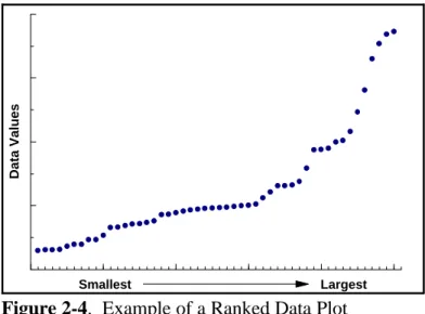
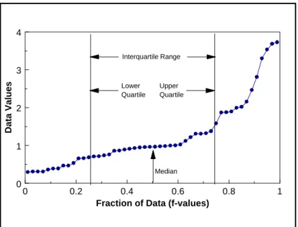
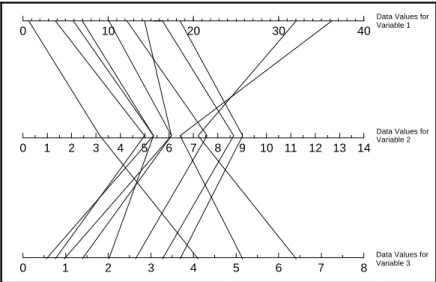
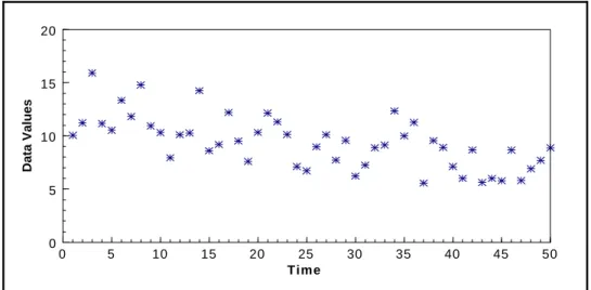
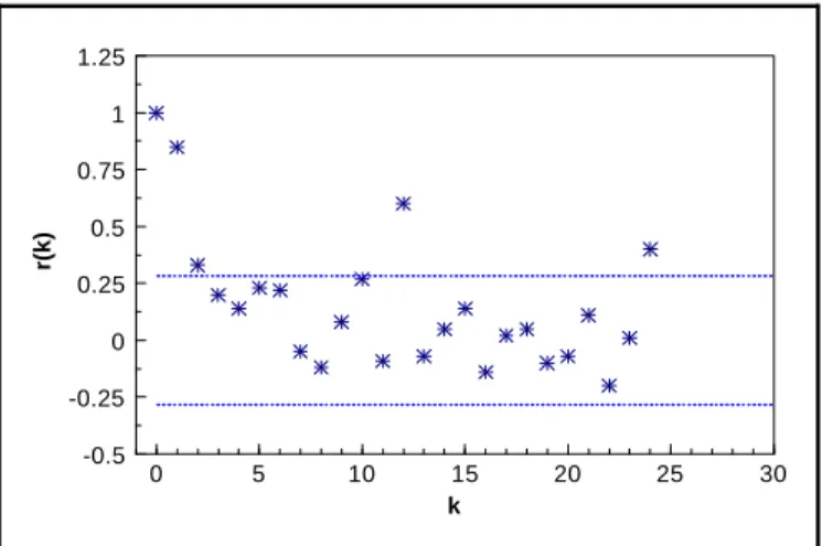
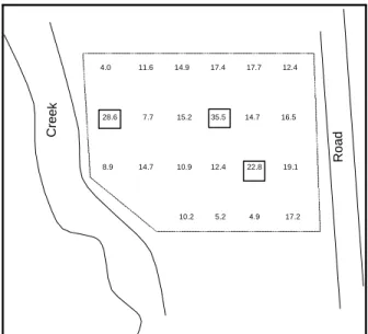
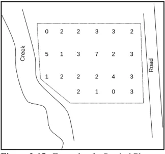
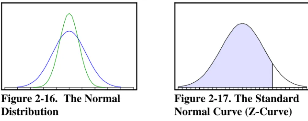
Figure 2-1. Example of a Frequency Plot . . . 2 - 13 Figure 2-2. Example of a Histogram . . . 2 - 14 Figure 2-3. Example of a Box and Whisker Plot . . . 2 - 17 Figure 2-4. Example of a Ranked Data Plot . . . 2 - 20 Figure 2-5. Example of a Quantile Plot of Skewed Data . . . 2 - 21 Figure 2-6. Normal Probability Paper . . . 2 - 25 Figure 2-7. Example of Graphical Representations of Multiple Variables . . . 2 - 26 Figure 2-8. Example of a Scatter Plot . . . 2 - 27 Figure 2-9. Example of a Coded Scatter Plot . . . 2 - 28 Figure 2-10. Example of a Parallel Coordinates Plot . . . 2 - 29 Figure 2-11. Example of a Matrix Scatter Plot . . . 2 - 29 Figure 2-12. Example of a Time Plot Showing a Slight Downward Trend . . . 2 - 33 Figure 2-13. Example of a Correlogram . . . 2 - 34 Figure 2-14. Example of a Posting Plot . . . 2 - 37 Figure 2-15. Example of a Symbol Plot . . . 2 - 38 Figure 2-16. The Normal Distribution . . . 2 - 40 Figure 2-17. The Standard Normal Curve (Z-Curve) . . . 2 - 40
EPA QA/G-9 Final
QA00 Version 2 - 3 July 2000
CHAPTER 2
STEP 2: CONDUCT A PRELIMINARY DATA REVIEW
2.1 OVERVIEW AND ACTIVITIES
In this step of DQA, the analyst conducts a preliminary evaluation of the data set,
calculates some basic statistical quantities, and examines the data using graphical representations. A preliminary data review should be performed whenever data are used, regardless of whether they are used to support a decision, estimate a population parameter, or answer exploratory research questions. By reviewing the data both numerically and graphically, one can learn the "structure" of the data and thereby identify appropriate approaches and limitations for using the data. The DQA software Data Quality Evaluation Statistical Tools (DataQUEST) (G-9D) (EPA, 1996) will perform all of these functions as well as more sophisticated statistical tests.
There are two main elements of preliminary data review: (1) basic statistical quantities (summary statistics); and (2) graphical representations of the data. Statistical quantities are functions of the data that numerically describe the data set. Examples include a mean, median, percentile, range, and standard deviation. They can be used to provide a mental picture of the data and are useful for making inferences concerning the population from which the data were drawn. Graphical representations are used to identify patterns and relationships within the data, confirm or disprove hypotheses, and identify potential problems. For example, a normal
probability plot may allow an analyst to quickly discard an assumption of normality and may identify potential outliers.
The preliminary data review step is designed to make the analyst familiar with the data. The review should identify anomalies that could indicate unexpected events that may influence the analysis of the data. The analyst may know what to look for based on the anticipated use of the data documented in the DQO Process, the QA Project Plan, and any associated documents. The results of the review are then used to select a procedure for testing a statistical hypotheses to support the data user's decision.
2.1.1 Review Quality Assurance Reports
The first activity in conducting a preliminary data review is to review any relevant QA reports that describe the data collection and reporting process as it actually was implemented. These QA reports provide valuable information about potential problems or anomalies in the data set. Specific items that may be helpful include:
• Data validation reports that document the sample collection, handling, analysis, data reduction, and reporting procedures used;
• Quality control reports from laboratories or field stations that document measurement system performance, including data from check samples, split samples, spiked samples, or any other internal QC measures; and
• Technical systems reviews, performance evaluation audits, and audits of data quality, including data from performance evaluation samples.
When reviewing QA reports, particular attention should be paid to information that can be used to check assumptions made in the DQO Process. Of great importance are apparent
anomalies in recorded data, missing values, deviations from standard operating procedures, and the use of nonstandard data collection methodologies.
2.1.2 Calculate Basic Statistical Quantities
The goal of this activity is to summarize some basic quantitative characteristics of the data set using common statistical quantities. Some statistical quantities that are useful to the analyst include: number of observations; measures of central tendency, such as a mean, median, or mode; measures of dispersion, such as range, variance, standard deviation, coefficient of variation, or interquartile range; measures of relative standing, such as percentiles; measures of distribution symmetry or shape; and measures of association between two or more variables, such as correlation. These measures can then be used for description, communication, and to test hypothesis regarding the population from which the data were drawn. Section 2.2 provides detailed descriptions and examples of these statistical quantities.
The sample design may influence how the statistical quantities are computed. The formulas given in this chapter are for simple random sampling, simple random sampling with composite samples, and randomized systematic sampling. If a more complex design is used, such as a stratified design, then the formulas may need to be adjusted.
2.1.3 Graph the Data
The goal of this step is to identify patterns and trends in the data that might go unnoticed using purely numerical methods. Graphs can be used to identify these patterns and trends, to quickly confirm or disprove hypotheses, to discover new phenomena, to identify potential
problems, and to suggest corrective measures. In addition, some graphical representations can be used to record and store data compactly or to convey information to others. Graphical
representations include displays of individual data points, statistical quantities, temporal data, spatial data, and two or more variables. Since no single graphical representation will provide a complete picture of the data set, the analyst should choose different graphical techniques to illuminate different features of the data. Section 2.3 provides descriptions and examples of common graphical representations.
At a minimum, the analyst should choose a graphical representation of the individual data points and a graphical representation of the statistical quantities. If the data set has a spatial or temporal component, select graphical representations specific to temporal or spatial data in addition to those that do not. If the data set consists of more than one variable, treat each variable individually before developing graphical representations for the multiple variables. If the