ATTRIBUTE ORIENTED INDUCTION
HIGH LEVEL EMERGING PATTERN
(AOI-HEP)
H L H SPITS WARNARS
ATTRIBUTE ORIENTED INDUCTION
HIGH LEVEL EMERGING PATTERN
(AOI-HEP)
HARCO LESLIE HENDRIC SPITS WARNARS
A thesis submitted in partial fulfilment of
the requirement of
the Manchester Metropolitan University
for the degree of Doctor of Philosophy
School of Computing, Mathematics and
Digital Technology
the Manchester Metropolitan University
2013
i
Acknowledgements
First of all I would like to acknowledge my PhD director of study and as first PhD supervisor, Dr. Maybin K. Muyeba for his time, patient, guidance, help and advice during my PhD study. I appreciate for the wisdom of his supervision, to find the research idea in second year of my PhD study, made me independent in my PhD research and gave me challenge in my research progression. He guided me in writing international conference papers,which were published in Lecture Notes in Computer Science (LNCS). I am also thankful to my reviewer Dr. Keeley A. Crockett for her constructive opinion on my PhD study. Thanks to the chair of my Viva Prof. Nicholas Bowring, internal examiner Dr. Liangxiu Han and second examiner Dr. M. Saraee for their input and improvement upon this thesis.
I thank the Research, Enterprise and Development (RED) office at Manchester Metropolitan University for supporting my PhD academic research skills with training and workshops. Also thanks to staff in the Research Degree Administration office, Faculty of Science and Engineering, Manchester Metropolitan University. They gave quick response when I encountered problems during the four years of my PhD study. Also, my acknowledgements go out to Indonesian government for the scholarship. Thanks to the chairman of Budi Luhur foundation Mr. Kasih Hanggoro, MBA.
I thank all my colleagues, Dr. Alma Adventa for her proof reading and help in writing, Dr. Gindo Tampubolon, Dr. Yanuar Nugroho, Dr. Delvac Oceandy and Dr. Danny Pudjianto for all PhD matters. Also thanks to Indonesian Students Association Greater Manchester for the friendships and cheerfulness. Thanks to Indonesian Fellowship Manchester for the spirit, care and prayer.
Finally, heartful thanks go to my family, my mum and dad, my parents in law, my wife Jen Nie for her delicious cuisines, my daughters Michell and Olivia, my sons Leonel, Laurens and Leandro for their patience, love and prayer.
ii
Abstract
Attribute-Oriented Induction of High-level Emerging Pattern(AOI-HEP) is a combination of Attribute Oriented Induction (AOI) and Emerging Patterns (EP). AOI is a summarisation algorithm that compact a given dataset into small conceptual descriptions, where each attribute has a defined concept hierarchy. This presents patterns are easily readable and understandable.Emerging patterns are patterns discovered between two datasets and between two time periods such that patterns found in the first dataset have either grown (or reduced) in size, totally disappeared or new ones have emerged. AOI-HEP is not influenced by border-based algorithm like in EP mining algorithms. It is desirable therefore that we obtain summarised emerging patterns between two datasets. We propose High-level Emerging Pattern (HEP) algorithm. The main purpose of combining AOI and EP is to use the typical strength of AOI and EP to extract important high-level emerging patterns from data.
The AOI characteristic rule algorithm was run twice with two input datasets,to create two rulesets which are then processed with the HEP algorithm. Firstly, the HEP algorithm starts with cartesian product between two rulesets which eliminates rules in rulesets by computing similarity metric (a categorization of attribute comparisons). Secondly, the output rules between two rulesets from the metric similarity are discriminated by computing a growth rate value to find ratio of supports between rules from two rulesets. The categorization of attribute comparisons is based on similarity hierarchy level. The categorisation of attributes was found to be with three options in how they subsume each other. These were Total Subsumption HEP (TSHEP), Subsumption Overlapping HEP (SOHEP) and Total Overlapping HEP (TOHEP) patterns. Meanwhile, from certain similarity hierarchy level and values, we can mine frequent and similar patterns that create discriminant rules.
We used four large real datasets from UCI machine learning repository and discovered valuable HEP patterns including strong discriminant rules, frequent and similar patterns. Moreover, the experiments showed that most datasets have SOHEP but not TSHEP and TOHEP and the most rarely found were TOHEP. Since
AOI-iii
HEP can strongly discriminate high-level data, assuredly AOI-HEP can be implemented to discriminate datasets such as finding bad and good customers for banking loan systems or credit card applicants etc. Moreover, AOI-HEP can be implemented to mine similar patterns, for instance, mining similar customer loan patterns etc.
iv
Contents
Acknowledgements Abstract Contents List of Tables List of Figures 1. Introduction 1.1. Motivations ... 1.2. Contributions ... 1.3. Organization of thesis ... 2. Literature Review 2.1. Introduction ... 2.2. Data Mining ... 2.2.1. Knowledge Discovery in Databases ... 2.2.2. Data Mining Methods ... 2.3. Attribute Oriented Induction ... 2.3.1. Concept Hierarchies ... 2.3.2. AOI characteristic and discriminant rules ... 2.4. Emerging Patterns ... 2.4.1. Growth rate and Jumping Emerging Patterns ... 2.4.2. EPs algorithms ... 2.5. Critical Analysis of Literatures and New Approach ... 2.6. Conclusion ...3. AOI-HEP Mining Framework
3.1. Introduction ... 3.2. AOI-HEP Framework ... 3.3. HEP definitions ... 3.3.1. TSHEP definition ... 3.3.2. TOHEP definition ... 3.3.3. SOHEP definition ... 3.4. HEP algorithm ... 3.5. Metric similarity ... i ii iv vii ix 1 1 4 5 6 6 6 9 10 11 12 14 18 19 20 25 29 30 30 30 33 33 34 34 34 36
v
3.5.1. Mining TSHEP, SOHEP and TOHEP ... 3.5.2. Mining Frequent pattern ... 3.5.3. Mining Similar patterns ... 3.6. HEP Growth Rate ... 3.7. Conclusion ...
4. AOI-HEP Experiments
4.1. Introduction ... 4.2. Preliminaries on datasets ... 4.3. Experiments ...
4.3.1. Composition SLV values for mining TSHEP, SOHEP and TOHEP ... 4.3.2. Composition SLV values for mining frequent patterns ... 4.3.3. Composition SLV values for mining similar patterns ... 4.3.4. Composition Growth rate values ... 4.4. Mining frequent patterns ... 4.4.1. Mining frequent patterns from TSHEP ... 4.4.2. Mining frequent patterns from SOHEP ... 4.5. Strong Discriminant rules from frequent patterns ... 4.6. Mining Similar patterns ... 4.6.1. Mining similar patterns from TOHEP ... 4.6.2. Mining similar patterns from SOHEP ... 4.7. Discriminant rules from similar patterns ... 4.8. Experiment’s analysis ... 4.8.1. AOI-HEP mining in adult dataset ... 4.8.2. AOI-HEP miningin breast cancer dataset ... 4.8.3. AOI-HEP mining in census dataset ... 4.8.4. AOI-HEP mining in IPUMS dataset ... 4.8.5. Experiment’s analysis conclusion ... 4.9. AOI-HEP justification... 4.10. Conclusion ... 5. Conclusion 5.1. Introduction ... 5.2. Summary ... 38 40 42 44 45 47 47 47 48 62 64 64 65 66 67 68 71 75 75 76 78 81 82 83 84 84 86 89 93 95 95 95
vi 5.3. Future research ... Publication list Appendices References 98 104 107 118
vii
List of Tables
4.1. Ruleset R2 for learning government concept from “workclass” attribute of adult dataset ... 4.2. Ruleset R1 for learning non government concept from “workclass”
attribute of adult dataset ... 4.3. Ruleset R2 for learning AboutAverClump concept from “clump
thickness” attribute of breast cancer dataset ... 4.4. Ruleset R1 for learning AboveAverClump concept from “clump
thickness” attribute of breast cancer dataset ... 4.5. Ruleset R2 for learning Green concept from “means” attribute of
census dataset ... 4.6. Ruleset R1 for learning Non Green concept from “means” attribute of
census dataset ... 4.7. Ruleset R2 for learning unMarried concept from “marst” attribute of
IPUMS dataset ... 4.8. Ruleset R1 for learning Married concept from “marst” attribute of
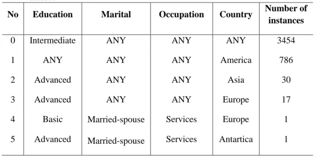
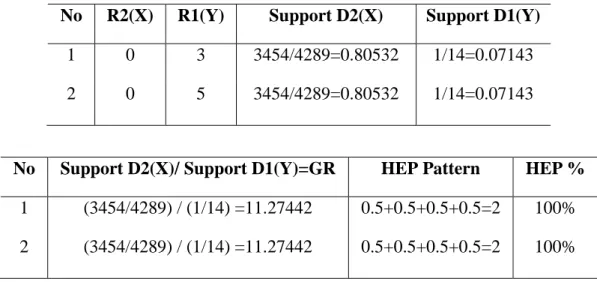
IPUMS dataset ... 4.9. TSHEP from adult dataset ... 4.10. SOHEP from adult dataset ... 4.11. SOHEP from breast cancer dataset ... 4.12. TSHEP from census dataset ... 4.13. SOHEP from census dataset ... 4.14. SOHEP from IPUMS dataset ... 4.15. TOHEP from IPUMS dataset ... 4.16. Composition SLV values for four experimental datasets ... 4.17. Composition Growth rate values for four experimental datasets ... 4.18. TSHEP in adult dataset for rulesets 1
3 R to 2
0
R with GR= (3454/4289) / (1/14) = 0.80532/0.07143= 11.27442 ... 4.19. TSHEP in adult dataset for rulesetsR15 to with
49 50 50 50 51 51 51 52 54 55 56 57 58 60 61 62 65 68 2 0 R
viii
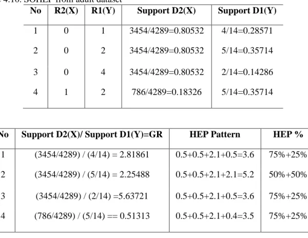
GR=(3454/4289)/(1/14)=0.80532/0.07143=11.27442 ... 4.20. Frequent subsumptionSOHEP in adult dataset for rulesets 1
1 R to with GR=(3454/4289)/(4/14)=0.80532/0.28571=2.81861 ... 4.21. Frequent subsumptionSOHEP in adult dataset for rulesets 1
4 R to
with GR=(3454/4289)/(2/14)=0.80532/0.14286=5.63721 ... 4.22. Frequent subsumptionSOHEP in breast cancer dataset for rulesets
to R22with GR=(19/533)/(1/289)=0.03565/0.00346=10.30206 ... 4.23. Frequent patterns for creating strong discrimination rules ... 4.24. TOHEP in IPUMS dataset for rulesets to with
GR=(6356/140124)/(2296/77453)=0.045/0.029=1.530 ... 4.25. TOHEP in IPUMS dataset for rulesets to with
GR=(4603/140124)/(5706/77453)=0.033/0.074=0.446 ... 4.26. Frequent overlapping SOHEP in breast cancer dataset for rulesets
to with GR=(5/533)/(4/289)=0.00938/0.01384=0.67777 ... 4.27. Frequent overlapping SOHEP in IPUMS dataset for rulesets to
with GR=(7632/140124)/(1217/77453)=0.05447/0.01571=3.46636 ... 4.28. Similar patterns for creating discrimination rules ... 4.29. Performance metric for number of rules resulted and time to process .. 4.30. Performance metric for features from current data mining techniques
AOI and EP ... 68 70 71 71 72 76 76 77 78 78 89 92 2 0 R 2 0 R 1 4 R
ix
List of Figures
2.1 Transformation of data to become patterns or models with data mining 2.2 Phases of the KDD methodology ... 2.3 A concept hierarchy tree for attribute workclass in adult dataset ... 2.4 A concept hierarchy for concept hierarchy tree attribute workclass in
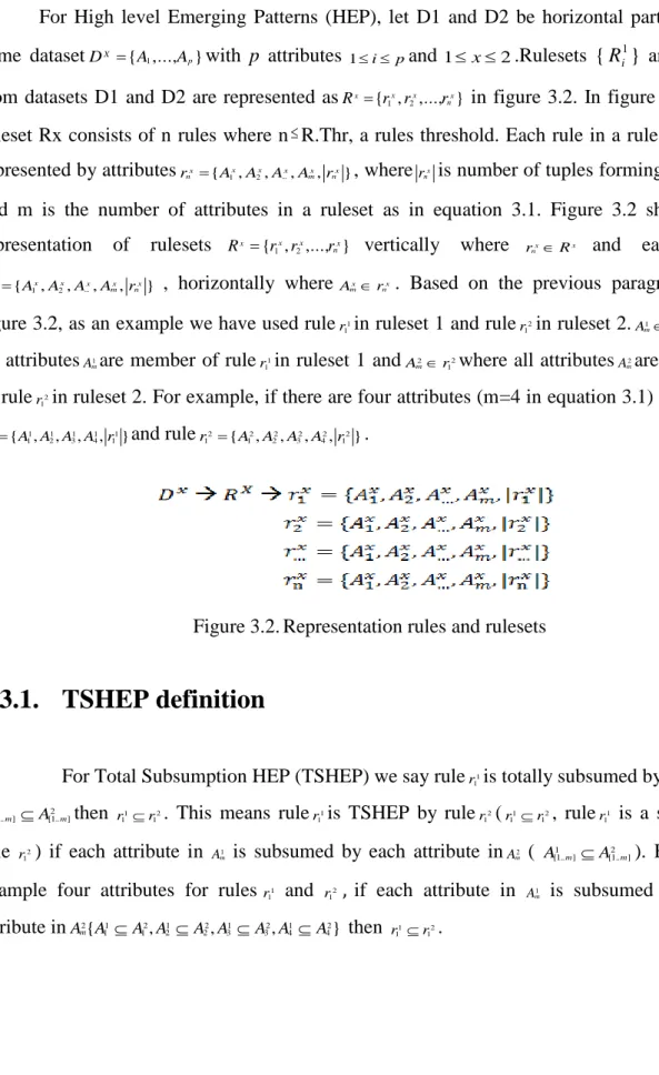
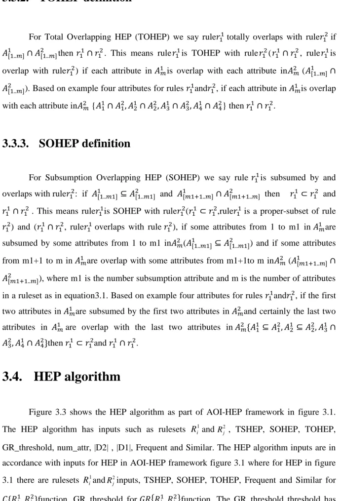
adult dataset ... 2.5 AOI characteristic and discriminant rules architecture ... 2.6 AOI characteristic rule algorithm ... 2.7 AOI discriminant rule algorithm ... 3.1 AOI-HEP Framework ... 3.2 Representation rules and rulesets ... 3.3 HEP algorithm ... 3.4 Comparing rule 1 of ruleset 2{ } and rule 1 of ruleset 1{ } ... 3.5 Composition subsumption and overlapping for mining patterns ... 4.1 Screen display for AOI-HEP application ... 4.2 Composition SLV values for four experimental datasets ... 4.3 Composition Growth rate values for four experimental datasets ... 4.4 AOI-HEP mining interest matrix ... 4.5 AOI-HEP Frequent pattern mining interest ... 4.6 AOI-HEP Similar pattern mining interest ... 4.3 AOI-HEP Frequent and Similar patterns mining interest ...
7 10 13 13 14 16 18 32 33 35 36 39 52 63 66 87 87 88 88
1.1.
Motivations
Recent developments in data minng show that single algorithms are no longer feasible to be used in isolation when looking for patterns that span different datasets, users and application. This research is motivated by a hybrid approach involving Attribute Oriented Induction (AOI) [30-48,55,58,61-63] and Emerging Patterns (EP) [65-72,75-84] that extracts high-level and emerging patterns, respectively from data. AOI was proposed in 1989 by Han and his colleagues [31], integrates a machine learning paradigm especially learning from examples technique with database operations, extracts generalized rules from an interesting set of data and discovers high-level data regularities. AOI uses concept hierarchy as background knowledge or taxonomies of every attribute domain. The attribute concepts are ordered level by level from specific (low-level) into general or higher level concepts. AOI then performs generalization of attribute values by ascending to the next higher level concepts along the paths of the concept hierarchy [40-42]. Meanwhile, Emerging Patterns (EP) was proposed in 1999 [80]. EP captures emerging trends when applied to time stamped datasets or capture useful contrasts between data classes when applied to datasets with classes. EP captures significant changes and differences between datasets defined as itemsets whose supports increase significantly from one dataset to another [67, 77]. The increasing of supports for itemsets from one dataset to another is called growth rate [67, 77].
The strength of AOI is in the use of concept hierarchies for generalization in order to generalize from low level data into high-level data. Moreover, AOI has been tested successfully against large relational datasets [44] and is able to learn different kinds of rules such as characteristic, discrimination, classification, data evolution regularities [39], association and cluster description rules[40]. Meanwhile, the strength of EP is in discriminating between datasets using growth rate functions (the ratio of the supports in one datasetD1 to another datasetD2 [75,79]. Combining AOI and EP proposes a technique that can strongly discriminate high-level data and learn different kinds of rules, thus creating a novel technique called Attribute-Oriented Induction High-level Emerging Pattern (AOI-HEP). This technique uses growth rate of patterns between datasets to discriminate high-level data resulting from concept hierarchy generalizations. Furthermore, this presents AOI-HEP as a new data mining framework relevant to the management level decision making process..
Previously, EP was proposed with border-based algorithm [79] and has had influences on other extended EP mining algorithms such as Classification by Aggregating EPs (CAEP) [84], information-based approach for Classification by Aggregating EPs (iCAEP)[67] and Classification by Aggregating Essential EPs (CAEEP)[100]. Others include Decision making by EPs (DeEP) [65], Bayesian Classification by EPs (BCEP)[78], Constrained Emerging Patterns (CEP) [77], Jumping Emerging Pattern classifier (JEP-Classifier)[83], JEP space[82], Knowledge Trends Data Analysis (KTDA)[89], Prediction by Likelihoods (PCL) [102] and Gtree[90]. Border-based algorithm avoid the long process naive algorithms do to get the counts of all itemsets in a large collection of candidates by manipulating only borders of some two collections and derive all EPs whose support satisfies a minimum support threshold [79]. Border-based algorithms define borders<L,R> where L is the sets of the minimal itemsets (superset or the most general EPs on the left) and R is the sets of the maximal itemsets (subset or the most specific EPs on the right) [71,72]. Border-based algorithm defines border <L,R> where each element L is a subset of some elements in Rand each element of R is a superset of some elements in L [79].
1. Differential procedure algorithm as part of border-based algorithm has to be called in multiple numbers of times when discovers all EPs [79].
2. Border-based algorithm has to be called twice when discovers all Jumping EP (JEPs) in both datasets (from target to contrasting datasets and vice versa) [70,78]. Meanwhile, Essential JEP (EJEP) and EJEP Classifier (EJEPC) use tree structure called Pattern-tree (P-tree) algorithm which efficiently mine EJEPs and EJEPCs in both datasets (from target to contrasting datasets and vice versa) without calling the algorithm twice [70,78].
The new AOI-HEP algorithm is not influenced by border-based approaches but is similar to comparisons with the decision tree technique CART-based method, which again, is not influenced by border-based algorithm. The CART-based approaches discover relevant EPs for classification using a CART tree [91].
AOI-HEP is similar to DeEP algorithm in terms of reduction the number of instances and attributes. DeEP was influenced by a border-based algorithm in EP to access low level data and has advantages on accuracy, speed and dimensional scalability over CAEP and JEP-C [83]. DeEP reduces number of instances and attributes from the training data with instance-based approach [65,72,81] whilst AOI-HEP uses AOI characteristic rule algorithm [30-31]. DeEP reduces the number of attributes with intersection operation using neighbourhood-based intersection method [65,72, 81] while AOI-HEP reduces number of attributes by attribute generalization and removal of redundant tuples as a second step [30-31]. Moreover, DeEP reduces number of instances by selecting the maximal itemsets from intersection operation [65,72,81] while AOI-HEP reduces number of instances with AOI generalization until distinct instances are less or equal to an instance threshold[30-31].
Moreover, this research is also motivated in the following ways and findings: 1. Total Subsumption HEP (TSHEP – those rules that are completely subsumed). 2. Subsumption Overlapping HEP (SOHEP – those rules that overlap and are
subsumed).
3. Total Overlapping (TOHEP – those rules that are completely overlapping). 4. Frequent patterns.
In this thesis, AOI-HEP has been successfully implemented using four large real datasets from UCI machine learning repository., and discovered TSHEP, SOHEP, TOHEP, frequent and similar patterns. The experiments showed that most datasets have SOHEP but not TSHEP and TOHEP, and the most rarely found were TOHEP. Frequent patterns that show synonymy with large pattern are interesting to be mined since with frequent patterns we can have strong discrimination, whilst similar patterns are interesting to be mined which can show equality of patterns that represent similar behaviours. The experiments showed that TSHEP tend to frequent patterns and TOHEP tend to similar patterns. Meanwhile, SOHEP occur between frequent and similar patterns (which are based on frequent similarity value i.e. the frequent similarity subsumption for frequent patterns and frequent similarity overlapping for similar patterns).
From frequent and similar patterns, we can create discrimination rules which show discrimination for each dataset influenced by learning high-level concepts in one of attributes of dataset. From frequent and similar patterns, we can get strong discriminant rules if the patterns have large growth rates where there are large supports in target dataset and small supports in contrasting dataset [69,71,79].
1.2.
Contributions
The main contributions of this thesis are:
1) Presenting a new framework that combines Attribute-Oriented Induction (AOI) and Emerging Pattern (EP).
2) Discriminating high-level data from two different rulesets which are from two different datasets.
3) Mining different types of High-level Emerging Patterns (HEP) i.e. Total Subsumption HEP (TSHEP), Subsumption Overlaping HEP (SOHEP) or Total Overlapping HEP (TOHEP).
.
5) Creating discriminant rules including strong discriminant rules from frequent and similar patterns.
6) Finding the interesting dataset to be mined for frequent and/or similar patterns.
1.3.
Organization of thesis
The rest of the thesis is organized as follows: Chapter 2 illustrates research literatures in data mining and in particular two data mining techniques, Attribute Oriented Induction (AOI) and Emerging Patterns (EP); In chapter 3, Attribute Oriented Induction High-level Emerging Pattern (AOI-HEP) mining framework is described and defines TSHEP, SOHEP and TOHEP including theory to mine TSHEP, SOHEP, TOHEP, frequent and similar patterns; Chapter 4 defines AOI-HEP experiments using four datasets from UCI machine learning repository [56] to mine TSHEP, SOHEP, TOHEP, frequent and similar patterns which can create discriminant rules. Finally, conclusion and possible future research are described in chapter 5.
2.1.
Introduction
This chapter presents an overview of the research literature in general of data mining and in particular two data mining techniques, Attribute Oriented Induction (AOI) and Emerging Patterns (EP). These data mining techniques are combined to propose a new algorithm called AOI-HEP. In the next section, we discuss data mining theory and discovery of patterns from data, the interestingness of discovery patterns, Knowledge Discovery in Databases (KDD) methodology and data mining algorithm (methods or techniques). Moreover, section 2.3 specifies the AOI data mining technique, kinds of knowledge rules that be can learned, concept hierarchy as AOI background knowledge and AOI characteristic and discrimination rules algorithms including eight generalization strategy steps. Furthermore, section 2.4 defines EP data mining technique which can captures the differences between classes, the support for class, growth rate, Jumping Emerging Pattern (JEP) and EPs algorithms include EP-based classifier for classification more than two classes. Meanwhile, section 2.5 illustrates the powerful AOI-HEP as combination AOI and EP data mining techniques, the differences between AOI-HEP and the famous border-based algorithm, similarity AOI-HEP with DeEP algorithm and previous researches which combining EP with other technique. Finally, the summary for this chapter is presented in section 2.6.
2.2.
Data Mining
Businesses need information which can be used as data for the decision making process. Data when used effectively can be very valuable in the competitive business world. On the other hand when data is not used effectively, it could be less competitive for a business. Data mining is useful for processing data and then extracting patterns that are valuable for decision making. For instance, customer patterns are valuable information for banking systems to secure bank loan and precious knowledge for retail systems to increase profit and customer loyalty. As shown in figure 2.1, the data mining algorithm is the process
of discovering patterns and models from data for the decision making. Data mining as a particular step in Knowledge Discovery in Databases (KDD) is a non trivial process of identifying valid, novel, potentially useful, and ultimately understandable patterns of the data [4]. Data mining uses specific algorithms such as discrimination, classification, association, clustering and etc. to produce different patterns and models. The discovered patterns should have the following criteria [1,4] :
1) Valid on new data with some degree of certainty.
2) Novelty where at least to the system and preferably to the user. 3) Usefulness that lead to some benefits to the users or for the tasks.
4) Understandable which can be estimated through simplicity, and if not immediately then after some post processing.
Figure 2.1.Transformation of data to become patterns or models with data mining
Discovery patterns or knowledge will yield many patterns and as the huge number of pattern are difficult to understand then elimination process can be applied with the use of threshold value, in order to find the most interesting patterns. The interestingness of discovered patterns is measured by combining the four patterns criteria such as validity, novelty, usefulness and simplicity for understandable estimation [16]. The two methods commonly used to find interesting pattern are [28] :
1) Subjective methods, which are user driven and domain dependent and for instance, the user should specify the rule to be considered interesting.
2) Objective methods, which are data driven and domain independent and for instance, the interestingness of rule depends on the quality of the rule and its similarity to other rules. The subjective and objective methods are similar with two types of KDD goals [1,4] and they are :
1) Verification, where the system is limited to verify the user’s hypothesis.
2) Discovery, where the system autonomously finds new patterns. The discovery goal is then subdivided into i.e.:
Data Patterns Models Data Mining Decision Making Human Business
2.a) Prediction, where the system finds patterns for predicting the future behaviour of some entities.
2.b) Description, where the system finds patterns for presentation to users in a human understandable form. Predictivemodels can be descriptive model and vice versa. As a scientific discipline, data mining intersects with other disciplines [2,4] i.e. databases, statistics, machine learning, Artificial Intelligence, expert system and pattern recognition, neural network, data visualization, information retrieval, image and signal processing, and spatial data analysis. Data mining has been applied for some real world problems in many industries such as spatial data mining, musical data mining, text data mining, visual data mining, privacy preserving data mining and etc [21]. In 2011 KDnuggets poll surveyed industries that have applied data mining in their operations and the top ten industries were Customer Relationship Management (CRM), banking, health care, education, fraud detection, science, social networks, credit scoring , direct marketing/fundraising and insurances[14].
Spatial data mining is a process of mining the knowledge from spatial data such as image and movie in order to find patterns. It has wide applications in Geographic Information Systems (GIS), remote sensing, image and video database, medical imaging, robot navigation, and etc[29]. Musical Data Mining use data mining techniques, including co occurrence analysis in order to discover similarities between songs and classify songs into correct genre’s or artists [24,25]. Meanwhile, text data mining where use of large online text collections to discover new facts and trends about the words itself[10-12]. Visual data mining apply data mining by using information visualization technology to improve data analysis [5]. Finally, in privacy preserving data mining is extended or preserved user privacy in order to letting the users to provide a modified value for sensitive attributes, where the modified value may be generated using custom code, a browser plug-in or extension to products in order to mask sensitive information [6-9].
Data mining is capable of handling the huge data overload problem as data continues to grow. KDnuggets poll showed the largest database/datasets that have been used with 21.4% voters used over 1 Terabyte database/dataset, 4% voters used over 1 Petabyte database/dataset and 19.5% voters used 1.1 to 10 Gigabyte database/dataset [19]. Data mining extracts knowledge from different kinds of databases e.g. relational databases, transaction databases, object oriented databases, deductive databases, spatial databases, temporal databases, multimedia databases, heterogeneous databases, active databases, legacy databases, and the internet information-base[3]. KDnuggets poll showed the most popular
data types to be mined in 2011, and the top ten were table data, time series, itemset/transactions, text (free-form), anonymized data, location/geo/mobile data, other, social network data, email and web content [17].
2.2.1.
Knowledge Discovery in Databases
The efforts in the industries mainly concern on the definition of methodologies that can guide the implementation of Data Mining applications. KDD as one of the most popular methodologies [22,23] has focus on the overall process of knowledge discovery from data, including store and access data, the efficient algorithms which deal with huge data, the interpretation and visualization of the knowledge discovery results. The term of KDD was coined in 1989 at the first KDD workshop [13]. As shown in figure 2.2., data mining as an essential step in KDD process consisting of an interactive and iterative of the following nine steps [1,4,13,27]:
1) Developing an understanding of application domain and identifying the goals of the KDD process from the customer’s viewpoint.
2) Creating a target dataset, selecting dataset and focusing on a subset of variables or data samples on which discovery is to be performed.
3) Data cleaning and pre processing, which include removing noise, collecting the necessary information, handling missing data fields and accounting for time sequence information as well as DBMS issues such as type, schema and mapping of missing and unknown values.
4) Data reduction and projection by finding the useful features to represent the data.
5) Matching the goals of KDD process in step one to particular data mining method through summarization, classification, regression, clustering and so on.
6) Exploratory analysis and model and hypothesis selection by choosing the data mining algorithm and selecting the method to be used for pattern searching.
7) Data mining by searching the patterns of interest in a particular representational form. 8) Interpreting the mined patterns which can also involve visualization of the extracted
patterns and models or visualization of the data given by the extracted models.
9) Acting the discovered knowledge by using the knowledge directly, incorporating the knowledge into another system for further action, or simply documenting it and reporting
it to the interested parties. This process also includes checking and resolving the potential conflicts with the previously believed (or extracted) knowledge.
Figure 2.2. Phases of the KDD methodology
2.2.2.
Data Mining Methods
There are many data mining methods/techniques/algorithms and a survey by KDnuggets showed the data mining algorithms which were used in 2011, and the top ten algorithms were decision tree/rules, regression, clustering, statistic (descriptive), visualization, time series/sequence analysis, support vector (SVM), association rules, ensemble methods and text mining [15]. Other survey showed the top ten algorithms were C4.5, K-Means, Support Vector Machine (SVM), Apriori, Expectation Maximization (EM), PageRank, AdaBoost, k-Nearest Neighbors (kNN), Naive Bayes and Classification and Regression Tress(CART) [20]. The following algorithms were in the top ten lists of both surveys i.e. decision tree/rules with C4.5, regression with CART, clustering with K-Means, support vector (SVM) with Support Vector Machine (SVM), association rules with Apriori, ensemble methods with Ada Boost.
Patterns Transformed Data Target Data Data Preprocessed Data Knowledge Selection Preprocessing Transformation Data Mining Interpretation/ Evaluation
Data mining algorithms tasks can be classified into [18,26] :
1) Supervised learning, with a known output variable in dataset and input labelled data which include classification, fuzzy classification, regression, decision tree, Support Vector Machine (SVM), artificial Neural Network, Naive Bayes and K-nearest Neighbor . 2) Unsupervised learning, without known output variable in dataset and input unlabeled data which include clustering,Expectation Maximization (EM), association rule and Self-Organizing Map (SOM).
A data mining algorithm should consists of three primary components [1,4] i.e. :
1) Model representation, where the language is used to describe discoverable patterns. 2) Model evaluation, where quantitative statements meet the goals of KDD process. 3) Search method, which consists of two components :
3.a) Parameter search, where the algorithm must search for the parameters, which optimize the model evaluation criteria, based on the observed data and fixed model representation.
3.b) Model search, where a loop occurs over the parameter search method.
2.3.
Attribute Oriented Induction
Attribute Oriented Induction (AOI) method was first proposed in 1989 integrates a machine learning paradigm especially learning-from-examples techniques with database operations, extracts generalized rules from an interesting set of data and discovers high level data regularities [31]. AOI provides an efficient and effective mechanism for discovering various kinds of knowledge rules from datasets or databases. The AOI method has been implemented in a data mining system prototype called DBMINER [36,37,43,45,55] which previously called DBLearn and been tested successfully against large relational database. DBLearn [32,38,62,63] is a prototype data mining system which was developed in Simon Fraser University. DBMINER was developed by integrating database, OLAP and data mining technologies [34,55].
AOI approach is developed for learning different kinds of knowledge rules such as characteristic rules, discrimination rules, classification rules, data evolution regularities [39], association rules and cluster description rules[40].
1) Characteristic rule is an assertion which characterizes the concepts which satisfied by all of the data stored in database. This rule provides generalized concepts about a property
that can help people to recognize the common features of the data in a class. For example the symptom of the specific disease [47].
2) Discriminant rule is an assertion, which discriminates the concepts of one (target) class from another (contrasting). This rule give a discriminant criterion which can be used to predict the class membership of of new data, for example to distinguish one disease from the other [47].
3) Classification rule is a set of rules, which classifies the set of relevant data according to one or more specific attributes. For example, classifying diseases into classes and provide the symptoms of each [30].
4) Association rule is association relationships among the set of relevant data. For example, discovering a set of symptoms frequently occurring together [35,50].
5) Data evolution regularities rule is general evolution behaviour of a set of the relevant data (valid only in time-related/temporal data). For example, describing the major factors that influence the fluctuations of stock values through time [33,41]. Data evolution regularities can then be classified into characteristic rule and discrimination rule [41]. 6) Cluster description rule is used to cluster data according to data semantics [50], for
example clustering the university student based on different attribute(s).
2.3.1.
Concept hierarchies
One advantage of AOI is that it has concept hierarchy as the background knowledge which can be provided by the knowledge engineers or domain experts [40,41,42]. Concept hierarchy stored a relation in the database provides essential background knowledge for data generalization and multiple level data mining. Concept hierarchy represents taxonomy of concept of the attribute domain values. Concept hierarchy can be specified based on the relationship among database attributes or by set groupings and be stored in the form of relations in the same database [45]. Concept hierarchy can be adjusted dynamically based on the distribution of the set of data relevant to the data mining tasks. The hierarchies for numerical attributes can be constructed automatically based on data distribution analysis [45]. Concept hierarchy for numeric will be treated differently for the sake of efficiency [58,59,60,61,64]. For example if there are a range of value between 0 and 1.99, then there willbe 199 values start from 0.00 until 1.99, but for efficiency there will be only 1 record created with 3 fields rather than with 200 records with 2 fields.
Charity Unemployed entrepreneur Centre Territory
Without-pay Never-worked Private Self-emp-not-inc Self-emp-inc Federal-gov State-Gov Local-gov
Non government Government
ANY
Figure 2.3. A concept hierarchy tree for attribute workclass in adult dataset[56]
Figure 2.4. A concept hierarchy for concept hierarchy tree attribute workclass in adult dataset[56]
In concept hierarchy, concepts are ordered by levels from specific or low level concepts into general or higher level. Generalization is achieved by ascending to the next higher level concepts along the paths of the concept hierarchy. The most general concept is the null description as the most specific concepts correspond to the specific values of the attributes in the database, which described as ANY. Concept hierarchy can be balanced or unbalanced, where unbalanced hierarchy then must be converted to a balanced hierarchy. Figure 2.3 shows the concept hierarchy tree for attribute workclass in adult dataset[56], which has three levels. The first level as the low level has 8 concepts and they are without-pay, never-worked, private, self-emp-not-inc, self-emp-inc, federal-gov,state-gov and local-gov concepts. The second level has 5 concepts and they are charity, unemployed, entrepreneur, centre and territory concepts. The third level as the high level has two concepts and they are non government and government concepts. For example, the concept of non government at the high level has 3 sub concepts in the second level: charity, unemployed and entrepreneur concepts. The concept entrepreneur at the second level has three sub concepts in the low level: private, self-emp-not-inc and self-emp-inc concepts. The concept hierarchy tree in figure 2.3 can be represented in figure 2.4 where symbol indicates generalization, for
Without-pay Charity
Never-worked Unemployed
{Private,self-emp-not-inc,self-emp-inc} entrepreneur {federal-gov,state-gov} Centre
Local-gov Territory
{Charity,Unemployed,entrepreneur} Non government
{Centre, Territory} Government
example, Without-pay Charity indicates that Charity concept is a generalization of Without-pay concept.
2.3.2.
AOI characteristic and discriminant rules
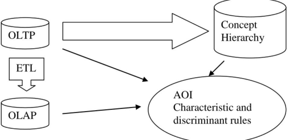
AOI can be implemented with an architecture design shown in figure 2.5 where characteristic rule and discriminant rule can be learned directly from the transactional database (OLTP) or Data warehouse (OLAP) [44,46] with the help of the concept hierarchy as the knowledge generalization. Concept hierarchy can be created from OLTP database as a direct resource.
Figure 2.5. AOI Characteristic and discriminant rules architecture
From a database, we can identify two types of learning:
1) Positive learning as the target class where the data are tuples in the database, which are consistent with the learning concepts. Positive learning/target class will be built when learn characteristic rule
2) Negative learning as the contrasting class in which the data do not belong to the target class. Negative learning/contrasting class will be built when learn discrimination or classification rule.
Characteristic rule has been used by AOI in order to recognize, learning and mining as a specific character for each of attribute as their specific mining characterization. Characteristic rule process the generalization with help of concept hierarchy as the standard saving background knowledge to find target class as a positive learning. Mining rule cannot be limited with just only one rule, as the more rules can be created the more mining can be
OLTP Concept Hierarchy OLAP ETL AOI Characteristic and discriminant rules
done. This has been proven as an intelligent system, which can help human to make a system that has ability to think like a human [3]. Rules often can be discovered by generalization in several possible directions [47].
Relational database as resources for data mining with AOI can be read with data manipulation language select sql statement [51,52,53,54]. Using a query for building rules gives an efficient mechanism for understanding the mined rules [49,50]. In the current AOI, a query is processed with SQL-like data mining query language DMQL at the beginning of the process [57].It collects the relevant sets of data by processing a transformed relational query, generalizes the data by AOI and then presents the outputs in different forms [45].
AOI generalizes and reduces the prime relation further until the final relation can satisfy the user expectation based on the set threshold. One or two thresholds can be applied, where one threshold is used to control both of number of distinct attributes and tuples in the generalization process, whilst two thresholds are used to control the number of distinct attributes and tuples in the generalization process. Threshold as a control for the maximum number of tuples of the target class in the final generalized relation can be replaced with group by operator in sql select statement which will limit the final result of generalization. Setting different threshold will generate different generalized tuples as the needed of global picture of induction repeatedly as time-consuming and tedious work [48]. All interesting generalized tuples as multiple rules can be generated as the global picture of induction by using group by operator or distinct function in the sql select statement.
AOI can perform datawarehouse techniques by doing generalization process repetitively in order to generate rules at different concepts levels in a concept hierarchy, enabling the user to find the most suitable discovery levels and rules. This technique performs rollup (progressive generalization [44]) or drill down (progressive specialization [44]) and operation [40,45] have been recognized as datawarehouse techniques. Finding the most suitable discovery levels and rules would add multidimensional views to a database using generalization process repetitively at different concepts level.
There are eight strategy steps that must be done [41] in the process of generalization. Here, step one until seven are for characteristic rule and step one to eight 8 are for discriminant rule.
1) Generalization on the smallest decomposable components, generalization should be performed on the smallest decomposable components of a data relation.
2) Attribute removal, if there is a large set of distinct values for an attribute but there is no higher level concept provided for the attribute, the attribute should be removed during generalization.
3) Concept tree Ascension, if there exists a higher level concept in the concept hierarchy for an attribute value of a tuple, the substitution of the value by its higher level concept would generalize the tuples.
4) Vote propagation, the value of the vote is the value of accumulated tuples where the vote will be accumulated when merging identical tuples in the generalization.
5) Threshold control on each attribute, if the number of distinct values in a resulting relation is larger than the specified threshold value, further generalization on this attribute should be performed.
6) Threshold control on generalized relations, if the number of tuples is larger than the specified threshold value, further generalization will be done based on the selected attributes and the merging of the identical tuples should be performed.
7) Rule transformation, change final generalization to quantitative rule and qualitative rule from a tuple (conjunctive) or multiple tuples (disjunctive).
8) Handling overlapping tuples, if there are overlapping tuples in both target and contrasting classes, these tuples should be marked and eliminated from the final generalized relation. AOI characteristic rule algorithm [41] is given as follow:
Figure 2.6. AOI characteristic rule algorithm AOI characteristic rule algorithm
Input: dataset, concept hierarchies, learning task, attribute threshold, rule threshold Output: characteristic rule of the learning task
1 For each of attribute Ai (1in, where n= # of attributes) in the generalized relation GR
2 { While #_of_distinct_values_in_attribute_Ai > threshold 3 { If no higher level concept in concept hierarchy for attribute_Ai 4 Then remove attribute Ai
5 Else substitute the value of Ai by its corresponding minimal generalized concept 6 Merge identical tuples
7 } 8 }
9 While #_of_tuples in GR > threshold 10 { Selective generalize attributes 11 Merge identical tuples
This AOI characteristic rule algorithm is the implementation of step one to seven of the generalization strategy steps. The algorithm shows two sub processes i.e. control number of distinct attributes and control number of tuples.
1) Control number of distinct attributes is a vertical process which checks every per attribute vertically. This is done by checking all attributes in the learning results of a dataset until the number of distinct attributes less equal than the threshold. This first sub process is just applied to the attributes which the number of distinct attributes greater than threshold. Each of attribute which the number of distinct attribute greater than threshold will be checked if it has a higher level concept in the concept hierarchy. If it has no higher level concept then the attribute will not be used. On the other hand if it has higher level concept then the attribute value will be substituted with the value of the higher level concept. Merging identical tuples will be done in order to summarize generalization and accumulate the value of the vote of the identical tuples by eliminating the redundant tuples. Eventually, after this first sub process all the attributes in generalization will have number of distinct attributes less equal than the threshold. This first sub process is implementation of step one to five of the generalization strategy steps.
2) Control number of tuples is a horizontal process, which checks per rule horizontally. This is carried out for those attributes, which passed the first sub process where each attribute will have the number of distinct attributes less equal than the threshold. This second sub process is only done while the number of rules is greater than threshold. Selective generalization of the attributes and merging of the identical tuples will reduce the number of rules. Selecting candidate attribute for further generalization can be done by preferences with finding the ratio on the number of tuples or the number of distinct attribute values. Selecting candidate attribute for further generalization can be examined by user based on the non interesting one, either non interesting attribute or non interesting rule. As with first sub process merging the identical tuples will be done in order to summarize generalization and accumulate the vote value of identical tuples by eliminating the redundant tuples. Eventually, after this second sub process the number of rules is less equal than the threshold. This second sub process is the implementation of step three, four and six of the generalization strategy steps.
AOI discriminant rule algorithm is the implementation of step one until eight of generalization strategy steps. Since AOI discriminant rule and AOI characteristic rule algorithms have the same generalization strategy steps between steps one and seven, then
literally they have the same process and the difference is just only in step eight. They also have the same sub processes i.e. control number of distinct attributes as the first sub process and control number of tuples as the second sub process. The step handling overlapping tuples as the eight generalization strategy step is process in the beginning before the first sub process and both in first and second processes before merge identical tuples.
AOI discriminant rule algorithm [39] is shown below:
Figure 2.7. AOI discriminant rule algorithm
2.4.
Emerging patterns
Emerging Patterns (EPs) as discovery knowledge from database capture emerging trends when applied in time stamped databases or capture useful contrasts between data classes when applied to datasets with classes[80]. Moreover, EPs capture significant changes and differences between datasets are defined as itemsets whose supports (frequencies) increase significantly from one dataset to another. The changing of supports for itemsets from one dataset to another (the ratios of the two supports) is called growth rates. Furthermore, EPs use user-defined threshold in order to reduce large candidate patterns, then can be said EPs are itemsets whose growth rates are larger than a given threshold. Finally, EPs are similar to discriminant rules or evolution rules in Attribute Oriented Induction (AOI) [40] but
AOI discriminant rule algorithm
Input: dataset, concept hierarchies, learning task, attribute threshold, rule threshold Output: discriminant rule of the learning task
1 For each of attribute Ai (1in, where n= # of attributes) in the generalized relation GR
2 { Mark the overlapping tuples
3 While #_of_distinct_values_in_attribute_Ai > threshold
4 { If no higher level concept in concept hierarchy for attribute_Ai 5 Then remove attribute Ai
6 Else substitute the value of Ai by its corresponding minimal generalized concept 7 Mark the overlapping tuples
8 Merge identical tuples 9 }
10 }
11 While #_of_tuples in GR > threshold 12 { Selective generalize attributes 13 Mark the overlapping tuples 14 Merge identical tuples
different since EPs do not limited by exclusiveness constraint and because the extra information of growth rate [79].
Those EPs with very large growth rates are notable differentiating characteristic between 2 datasets and have been useful for building powerful classifiers [69,79]. Thus, Those EPs with very large growth rates are frequent in one class but rare in another class. Meanwhile EPs with low to medium support such as 1% until 20% can give very useful new insights and guidance to experts, in even “well understood” applications [79]. Hence, the low supports EPs such as 0.1 until 5% may be new knowledge to the dataset and discover small support EPs is interesting [79]. The interestingness of discovery small support EPs due to reason too many EPs candidates and make naive algorithms too costly to examine all itemsets in dataset. For example if there are 350 itemsets in dataset then naive algorithm would need to process 2350 (Cartesian product) itemsets in order to find their supports in datasets D1 and D2 and then determine their growth rates.
2.4.1.
Growth rate and Jumping Emerging Patterns
Let I = {i1,i2,...,iN} be a set of items. A dataset is a set D of transactions. An itemset X
is a subset of I. The support of an itemset X in a dataset D, denoted as suppD(X) in equation
2.1. suppD(X)= | | ) ( D X countD (2.1)
where : suppD(X) = support in dataset D containing itemset X
countD(X) = the number of transactions in dataset D containing itemset X
where countD(X) = t D and X t, where t is instance in D
= total number of instances in dataset D D = Dataset
X = Itemset or pattern
Given a positive number σ, we say an itemset X is σ-large in dataset D if suppD(X) ≥ σ, and
X is σ-small in dataset D otherwise. Assume there are given an ordered pair of datasets D1 and D2 then growth rate of an itemset X from datasets D1 to D2 denoted in equation 2.2 as GrowthRateD1D2(X) =
if suppD1(X)≠0, = 0 if suppD1(X)=suppD2(X)=0, and = ∞ if suppD1(X)=0≠suppD2(X). For EPs are associated with two datasets, dataset D1 will be called
background dataset or can be called negative class of the EPs and dataset D2 will be called target dataset or can be called positive class. Given ρ> 1 as growth rate threshold, an itemset X is said to be an ρ-emerging pattern (ρ-EPs or simply EPs) from D1 to D2 (sometimes states as an EPs in/of D2) if GrowthRate(X)≥ρ.
GrowthRate(X) = { } (2.2)
where : = infinity, when , Jumping EPs (JEPs)
suppD1(X) = support in dataset D1 containing itemset X (equation 2.1) suppD2(X) = support in dataset D2 containing itemset X (equation 2.1)
Jumping EPs (JEPs) are special EPs and also special discriminant rule whose supports increase abruptly from zero support in one dataset to non-zero support in another. JEPs is EPs with infinite (∞) growth rate value whose support is zero in dataset D1 (suppD1(X)=0) and
support is non-zero in dataset D2 (suppD2(X)≠0). For discovering JEPs, HORIZON-MINER
algorithm is used to find the large border (horizontal border) of all itemsets with non-zero support and MBD-LLBORDER is used to find JEPs using the two large borders derived by HORIZON-MINER as inputs [79]. Tree-based algorithms for computing JEPs that are 2
until10 times faster than previous methods, which combination two novel features [75] : 1) Tree-based data structure for storing the raw data which is similar to Frequent Pattern
(FP-tree) [73,74].
2) Development of a mining algorithm operating directly on the data contained in the trees.
2.4.2.
EPs algorithms
There are a lot of EPs algorithms and the previous algorithms border-based MBD-LLBORDER algorithm and ConsEPMiner. The EP mining with border-based
MBD-LLBORDER algorithm avoid the long process naive algorithms to get the counts of all itemsets
in a large collection of candidates, by manipulating only borders of some two collections and derive all EPs whose support satisfies a minimum support threshold in dataset D2 [79]. The border-based MBD-LLBORDER algorithm discovers all EPs by calling differential procedure
Miner that utilize two types of constraints (support and growth rate treshold) which efficiently mining EPs and use another constraint called growth rate improvement to eliminate the uninteresting EPs [68]. Beside three external constraints (support, growth rate and growth rate improvement), there are another three inherent constraint which are not user given, namely same subset support, top growth rate and same origin.
The EPs algorithms has been extended to classification called EP-based classifier where the process of finding a set of models can describe and distinguish between two or more data classes or concepts. For handling classification where distinguish more than 2 classes then each instance in dataset D is associated with p class labels: C1,C2, ...,Cp and partition dataset
D into p sets: D1,D2, ...,Dp with Di containing all instances of class Ci.
There are many EP-based classifier and they are: 1) Classification by Aggregating EPs (CAEP).
Its first application for EPs classification, employs ConsEPMiner algorithm and has three steps [84]:
1.a) For each class C, all the EPs meeting some support and growth rate thresholds, from the opponent set of all none-C instances to the set of all C instances.
1.b) Aggregating the power of the discovered EPs for classifying an instance s. Aggregating differentiating score for each class C by summing the differentiating power of all EPs of class C that occur in instance s.
1.c) Normalizing score for class C by dividing it by some base score of the training instances of class C.
The accuracy and performance CAEP can be improved with Score Behaviour Knowledge Space (SBKS) which to record the behaviour of training data on scores to make final classification decision. SBKS is an m-dimensional space where each dimension corresponds to the score of the class [66].
2)
Information-based approach for classification byaggregating EPs (iCAEP).A variant of CAEP and compare to CAEP, iCAEP has better predictive accuracy and shorter time for training and classification [67].
3) The Decision making by EPs (DeEP).
DeEP is instance-based classifier which makes decisions through EPs [65,72,81]. As a lazy EP-based classifier, instance-based approach creates remarkable reduction on both volume (the number of instances) and dimension (the number of attributes) of the training
data. DeEPs have advantages on accuracy, speed and dimensional scalability over CAEP [84] and JEP-Classifier [83].
DeEPs need three main steps to determine the class of a test instance: 3.a) Discovering border representation of EPs.
The step aims to learn discriminating knowledge from training data, reducing the data and discovering all JEPs. Assume we have classification set Dp={P1,...,Pm} of
positive instances and set Dn={N1,...,Nn} of negative instances.
3.b) Selecting the more discriminating EPs.
Since the number of JEPs is usually large then the most general JEPs among all JEPs will be reduced. By the most general JEPs is mean that the proper subsets are not JEPs anymore.
3.c) Determining collective scores based on the selected EPs for classification.
Determine the collective score of T instance for any specific class C by aggregating the supports of the selected EPs in class C using compact summation method. 4) Bayesian Classification by EPs (BCEP).
As a hybrid of the EP-based classifier and Naive Baiyes (NB) classifier[71,78] is superior than CAEP. There are 2 kinds of interesting EPs when mining with BCEP and they are : 4.a) Essential EPs (eEP), are EPs with very large growth rate (typically more than 1000),
enough(large) supports in the target class (usually threshold 1%) and that are contained in the left bound of the border representing EPs collection. Large growth rate show sharp discriminating power, large supports show enough coverage on the training dataset which EPs are more resistant to noise
4.b) Essential JEPs (EJEP) [70], are subset of JEPs which removing JEPs that contain noise and redundant information.
BCEP utilize tree-based algorithm [75] to efficiently mine the complete eEP and EJEP for each class.
5) Constrained Emerging Patterns (CEP).
CEP the same with border based MBD-LLBORDER algorithm [83] to find itemsets which support ≥α threshold in target (D2) dataset and support ≤ β threshold in background (D1) dataset [76,77]. CEP mining can be accomplished by an extension of JEP mining in two steps. Step 1 is to represent border based algorithm where one border represent target (D2) dataset with support ≥α threshold and the other border represent background (D1) dataset with support ≥ β threshold. Method for mining JEPs can be applied, once the borders are computed to gain the desired patterns in the next step [77].
Thereafter, step two is to mine the CEP by operating on the relevant borders. When β=0, CEP become JEP and when β>0 will have greater robustness CEP. Pair-wise classification strategy is used to mine CEP with more than two datasets, where each of dataset will be treated as target class and will be compared with unioning other datasets. For example CEP for dataset D1 are found by comparing D1 against the background dataset D2 D3... Dn. The CEP for dataset D3 are found by comparing D3 with respect to the background dataset D1D2D4....Dn etc.
For handling JEP, there are many EP-based classifier and they are : 1) JEP-Classifier (JEP-C).
JEP-Classifier is JEPs classification which partially influenced by CAEP and uses exclusively JEPs. JEP-Classifier uses datasets with more than two classes in an ordered way with pair-wise feature concept [83]. JEP-Classifier utilize border based
MBD-LLBORDER algorithm to discover border of all JEPs in order to identify the most expressive
JEPs. Border based MBD-LLBORDER algorithm is used to find JEPs in large databases and
using semi naive JEPPRODUCER algorithm to find JEPs in small databases. The most
expressive JEPS is the most frequency JEPs with large support that build accurate classification. The most expressive JEPs is the left bounds of the border.
2) JEP spaces.
JEP space with respect to target (D2) dataset and background (D1) dataset is defined as the set of all JEPs from background(D1) to target (D2) datasets (
). JEP space is collection where element only occurs in target dataset but not in background dataset [72]. JEP space satisfies the property of convexity and can be represented by two bounds, left bound and right bound, consisting respectively of the most general JEPs and the most specific JEPs [72,82]. There are 3 border operations for algorithm maintaining JEP spaces and they are :
2.a) Border difference (-).
Border difference is similar with MBD-LLBORDER algorithm [79] and using BORDER
-DIFF algorithm [79] with a slight different in output. The same like inputs for JEPPRODUCER algorithm [83], JEP space is represented with two horizontal borders
(horizontal spaces or convex space) from datasets D1 of positive instances denoted <{Ø},R1> and D2 of negative instances denoted <{Ø},R2>. In other words, JEP
space is represented with border <L,R> which have 2 bounds, they are Left bound/the most general JEPs/positive instances/<{Ø},R1> and Right bound/the most
specific JEPs/negative instances/<{Ø},R2>. Horizontal border or horizontal space is
non-zero support itemsets in the dataset. JEP space to D1 and D2 is present the set difference [{Ø},R1] - [{Ø},R2], where is subtracting all non-zero support itemsets in
dataset D2 from all non-zero support itemsets in dataset D1. 2.b) Border union (υ).
Border union is union of old JEP space and some JEP space created by new data. Suppose old JEP spaces D1 and D2 are positive and negative instances respectively.
Assume a set i1 (iR1) of new positive instances are inserted then JEP space (D1+i1)
and D2 or new JEP space is the union of the previous JEP space and a JEP space
associated with i1. Insertion of new Left bound/the most general JEPs/positive instances/<{Ø},R1> has set: ([{Ø},R1] υ [{Ø},iR1] ) - [{Ø},R2] = ( [{Ø},R1] -
[{Ø},R2] ) υ ( [{Ø},iR1] ) - [{Ø},R2] )
2.c) Border intersection (∩).
Border intersection is intersection of old JEP space and some JEP space created by new data. Suppose old JEP spaces D1 and D2 are positive and negative instances
respectively. Assume a set i2 (iR2) of new negative instances are inserted then JEP
space D1 and (D2 +i2) or new JEP space is the intersection of the previous JEP space
and a JEP space associated with i2. Insertion of new Right bound/the most specific JEPs/negative instances/<{Ø},R2> has set: [{Ø}, R1] – ([{Ø},R2] υ [{Ø},iR2])=(
[{Ø},R1] - [{Ø},R2] ) ∩ ( [{Ø}, R1] ) - [{Ø},iR2] )
3) Essential JEP (EJEP) and EJEP-Classifier (EJEP-C).
EJEP is discrimination between two classes and EJEP-Classifier (EJEPC-C) is classification for more than two classes by aggregating EJEPs with adopting pair-wise features concept. EJEP-C uses two parameters: the minimum support threshold and the percentage of top ranking items used for mining EJEPs. EJEP uses tree structure called Pattern-tree (P-tree) algorithm to mine EJEPs and the method advantage is a single-scan algorithm which efficiently mine EJEPs of both data classes (from D1 to D2 and from D2 to D1) at the same time [70,78]. Whilst border-based and ConsEPMiner algorithms will call the algorithm twice using target classes D2 and D1 separately.
2.5.
Critical Analysis of Literatures and New Approach
AOI and EP have been recognized as powerful mining technique in order to extract important knowledge from data. For level data processing, AOI usually are represented at high abstraction level in the concept hierarchy but EP concerns to distinguish properties at low conceptual level. AOI is recognized as a powerful mining technique since has been tested successfully against large relational database [44] and can learn different kinds of rules [39]. Process of generalization steps in AOI which produce high level data based on concept hierarchy as background knowledge, become the typical strength of AOI. Moreover, EP is recognized as a powerful mining technique to discriminate datasets [75,79]. Growth rate as ratio of the supports in one dataset to another dataset is justification for powerful discrimination, become the typical strength of EP. The main purpose to combine AOI and EP become AOI-HEP is to use typical strength of AOI and EP.
AOI-HEP unite the powerful AOI and EP by applying growth rate as a standard function in EP and using concept hierarchy as background knowledge in AOI. AOI-HEP apply growth rate for ratio of the supports at the same or different high level itemsets instead of the same low level itemsets as used in EP. Mining high level data with EP was ever proposed by:
1) Using brute-force approach with optimisations to mining generalised EPs called GTree algorithm[90]. GTree algorithm was influenced with border-based algorithm and a pattern is considered an EP if superset EP in Left border and has leaf-level as subset in Right border[90].
2) Using local-recording algorithm to hide sensitive information that is EPs in dataset for Privacy Preserving Data Publishing (PPDP) purposes and recoding is a process of grouping existing values to some new generalized values from concept hierarchies [104]. The algorithms is measuring the reduction of growth rate EPs with recording all attributes in frequent itemsets and hide all EPs with a minimal distortion in frequent itemsets [104]. Therefore, AOI-HEP as a new technique has powerful distinguishing features between datasets at high abstraction level. HEP can mines frequent and similar patterns. AOI-HEP proved to learn knowledge rules such as discriminant rule from frequent and similar patterns. AOI-HEP is influenced with EP which is recognized closely relate to frequent pattern[89] and in EP, patterns will be recognized as EP if patterns have a high support (frequent) in one class and low support (infrequent) in other one[71,89].
EP was proposed with border-based algorithm [79], which influences most other EP mining algorithms such as CAEP[84], CAEEP [100], DeEP[65], BCEP[78], CEP[77], JEP-C[83], JEP space[82] as EP-based classifier[103] algorithm, KTDA[89], PCL [102] and GTree [90] algorihtms. Border-based algorithm influences many other algorithms by implementing the border-based algorithm in their algorithms. Border-based algorithm define border <L,R> where L is the sets of the minimal itemsets (superset or the most general EPs) and R is the sets of the maximal itemsets (subset or the most specific EPs) [71,72]. Border-based algorithm defines border <L,R> where each element L is a subset of some elements in Rand each element of R is a superset of some elements in L [79].
AOI-HEP is not influenced by border-based algorithm and the differences between AOI-HEP and border-based algorithm are :
1) Border-based algorithm which influence EP-based classifier such as CAEP,DeEP, BCEP, JEP-C can do classification task by learning more than two datasets. Whilst AOI-HEP not yet implemented, but future research needs to be undertaken to extend AOI-HEP ability by learning more than two datasets in order to mine not only classification task, but other knowledge rules such as association rule, data evolution regularities and cluster description rules. Moreover, other future research in order to find interested HEP in AOI-HEP, the discovery is not just only from D1 to D2 datasets, but will be extended from D2 to D1 datasets as refer in the third step of discovery the interesting EPs in DeEP [65,72,81].
2) AOI-HEP discovers high level pattern instead of low level pattern in border-based algorithm.
3) AOI-HEP will have less High level EP (HEP) because of discovery in high level as cartesian product between rulesets. Whilst border-based algorithm will have the huge number of EPs because of discovery in low level.
4) AOI-HEP uses similarity hierarchy level and value between attributes in rules and growth rate threshold to reduce the number of HEP. However, border-based algorithm uses border and growth rate threshold to reduce the huge number of EPs, which consists the minimal and maximal EPs [80].
5) AOI-HEP discovers with the same or different itemset, but border-based algorithm with the same itemset.
6) There is no infinite (∞) growth rate or Jumping High level EP (JHEP) in AOI-HEP since all rules (high level pattern) in the ruleset have number of instances. Whilst in