IDENTIFICATION OF AN ELECTRICALLY DRIVEN MANIPULATOR
USING THE DIFFERENTIAL FILTERS – INPUT ERROR METHOD
Leszek CEDRO*
*Kielce University of Technology, Faculty of Mechatronics and Machinery Design, Al. Tysiąclecia PP 7, 25-314 Kielce, Poland [email protected]
Abstract: The paper presents an example of solving the parameter identification problem in case of robot with three degrees of freedom has been presented. The identification has been performed with the use of elaborated differential filters. The applied identification method does not require differential equations solving but only determining the appropriate derivatives. Identification method and its generaliza-tions using the object inverse model require information on time derivatives of the input and output signals. The required derivative order depends on the order of differential equations describing the object.
Key words: Differential Filters, Identification, Input Error Method
1. INTRODUCTION
The rapid developments in computer hardware and software and, consequently, the common use of computers to control processes have aroused wide interest in mathematical modeling, control processes and, accordingly, control system identification.
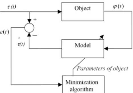
The method of identification applied in the analysis involves fi-ne-tuning of the inverse model. The method can be used only for such values of the input signals that are determined from the measurement data. Identifying a dynamic system by means of the input error method (Fig. 1) requires looking for a model that gen-erates the same input as the object. Only in the case of model reversibility is such a procedure possible. This reversibility is true for linear minimum-phase models and a certain class of non-linear models where the input is determined basing on the output data (Cedro and Janecki 2009; Cedro and Janecki 2011).
Let us assume, for instance, that the object is described by means of a differential equation:
τ
θ
ϕ
ϕ
ϕ
, − ,..., , )= ( (n) (n 1) f (1)where is a certain known function, unknown parameters and input signal. Thus, the identification error is defined as:
τ τ− ˆ = e , ) ˆ , ,..., , ( ˆ
ϕ
( )ϕ
( 1)ϕ
θ
τ
= n n− f (2)where ̂ estimate input signal and estimate unknown parame-ters.
A drawback of this method is that derivative estimates need to be determined. An advantage, on the other hand, is that it is not necessary to solve the differential equations describing the model at each step of iteration.
The fundamental problem related to the implementation of the input error method and its generalization is the necessity to de-termine the estimates of signal derivatives. This is achieved by applying differential filters (Janecki and Cedro 2007).
Fig. 1. Schematic diagram of the identification process
2. DIFFERENTIAL FILTERS
Let us assume that the differential filter of the k-th order is a series connection of a low-pass filter with boundary frequency Ω and a difference quotient of the k-th order (Fig. 2).
Fig. 2. Block diagram of the differential filter
The low-pass filter will be responsible firstly for reducing the signal spectrum and secondly for correcting the characteristics of the difference quotient in the range of low frequencies. Thus, the filter will be called a low-pass correction filter. The desired transfer function of the low-pass filter is:
Ω > Ω Ω ≤ Ω Ω Ω = Ω ∇ . for 0 for ) ( ) ( ) ( kor g g k k k H H H (3)
As a result, the transfer function of the series connection of the difference quotient and the low-pass filter in the range of low frequencies will be equal to the transfer function of an ideal differential filter.
Identification of an Electrically Driven Manipulator Using the Differential Filters – Input Error Method to: = Ω + Ω − Ω = Ω − Ω = Ω Ω = = Ω Ω = Ω ∇ . 3 )) 2 sin( sin 2 /( 2 ) cos 1 ( 2 / 1 sin / ) ( / ) ( ) ( 3 2 kor k k k H H H k k k (4)
The filter impulse response is the inverse Fourier transform of its frequency characteristic, thus:
∫
Ω Ω − Ω Ω Ω = g g d e H n h k k( ) j n 2 1 ) ( kor korπ
. (5)Unfortunately, integral (5) cannot be expressed by means of the analytic functions. It needs to be determined using some approximation. By expanding function (Ω) into a Taylor series around the value Ω = 0, we obtain:
= Ω + Ω + = Ω + Ω + = Ω + Ω + = Ω . 3 ) ( 4 1 2 ) ( 12 1 1 ) ( 6 1 ) ( 4 2 4 2 4 2 kor k O k O k O H k (6)
The four-term approximation of the expansion appears to be fairly sufficient. The inverse Fourier transform of the function obtained by rejecting the terms of the higher orders is equal to:
= Ω − Ω + + + Ω Ω = Ω − Ω + + + Ω Ω = Ω − Ω + + + Ω Ω = . 3 )) sin( ) 2 4 ( ) cos( 2 ( 4 1 2 )) sin( ) 2 12 ( ) cos( 2 ( 12 1 1 ) sin( ) 2 6 ( ) cos( 6 12 ) ( 2 2 2 3 2 2 2 3 2 2 2 3 kor k n n n n n n k n n n n n n k n n n n n n n h g g g g g g g g g g g k π π π (7)
Assume that the impulse response of the low-pass differential filter is: ) ( ) ( 1 ) (n hkor nWHarris n h k k k d = χ , (8)
Where () is Harris window described by the following equation: ). / 3 cos( 01 . 0 ) / 2 cos( 14 . 0 ) / cos( 49 . 0 36 . 0 ) ( Harris M n M n M n n W π π π + + + + = (9) The parameter should be selected in such a way that the slope of the characteristic of the filter being designed at point
0
=
Ω be the same as that of the ideal differential equation, thus:
k k k k d k k k j H H ∆ = Ω Ω Ω ∂ ∂ = Ω ∇ ( )| ! ) ( 0 . (10)
3. A MATHEMATICAL MODEL OF A ROBOT MANIPULATOR In the next sections, the following problems will be solved: first, we will derive the equations for the DC motors, then, we will define the kinetic and potential energy of the system, and finally, we will symbolically derive the robot dynamic equations, using the second order Lagrange equations.
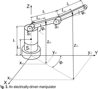
Fig. 3. An electrically-driven manipulator
Let = [] denote the vector of joint variables acting as generalized coordinates, ! – the mass, "! – the arm length, "#$ – the distance from the centre of gravity and %! – the motor of the link &.
Using typical equivalent diagrams of DC motors available in the literature, e.g. (Kowal, 2004), and the second Kirchoff law, we can write the following electrical equation of the DC motor:
j j j j R L e z U U E U = + + , for j=1,2,3 (11)
where '($ is the voltage supplied to the rotor.
Since an open-loop system may be difficult to control, it is es-sential that the identification be performed for a closed-loop sys-tem with properly selected PD controllers. Let us assume that the equations of the controllers have the following form:
) ( )) ( ) ( ( t t K t K Uz p z j d j j j j j = ϕ −ϕ − ϕ& , (12)
where: )*$, )+$ – the parameters of the controllers, ,$(-) – the control signals, !(-) – the variables describing the position of the manipulator arms.
The voltage drops across the rotor winding resistance and in-ductance are: ) (t i R U j j j w w R = , and (13) dt t di L U wj j j L ) ( = , (14)
where ./$ is the equivalent rotor winding resistance, 0! is the equivalent rotor winding inductance, and 1/$ is the current flow-ing through the rotor windflow-ings.
) (t k Ee e j j j = ϕ& , (15)
where 23$ is an electromotive constant.
Substituting the subsequent components to Eq. (11), we ob-tain: ) ( )] ( ) ( [ ) ( ) ( ) ( t K t t K t k t i R dt t di L j d j z p j e w w w j j j j j j j j ϕ ϕ ϕ ϕ & & − − = = + + , for j=1,2,3. (16)
The rotor torque is: ) (t i k M j j j m w s = , (17)
where 24$ is a mechanical constant.
Let us define the manipulator kinetic and potential energy. The following geometrical relations take place:
)) ( cos( )) ( cos( 2 1 2 l 2 t t xc = c
ϕ
ϕ
, )) ( cos( )) ( ) ( cos( )) ( cos( )) ( cos( 1 3 2 1 2 2 3 3 t t t l t t l xc cϕ
ϕ
ϕ
ϕ
ϕ
+ + + = , )) ( sin( )) ( cos( 2 1 2 l 2 t t yc = cϕ
ϕ
, )) ( sin( )) ( ) ( cos( )) ( sin( )) ( cos( 1 3 2 1 2 2 3 3 t t t l t t l yc cϕ
ϕ
ϕ
ϕ
ϕ
+ + + = , (18) )) ( sin( 2 1 2 l l 2 t zc = + cϕ
, )) ( ) ( sin( )) ( sin( 2 2 3 2 1 3 l l t l3 t t zc = +ϕ
+ cϕ
+ϕ
.The velocity of the centre of gravity of the second arm of the manipulator is: , 2 2 2 2 2 2 2 xc yc zc
v = & + & +&
. 2 3 2 3 2 3 3 xc yc zc
v = & + & + & (19)
Thus, the kinetic energy of the system is:
3 2 1 E E E E= + + , (20) 2 ) ( 2 1 1 1 t J E = cϕ& , 2 ) ( 2 2 2 2 2 2 2 2 t J v m E = + c ϕ& , 2 ) ( 2 2 3 3 2 3 3 3 t J v m E = + c ϕ& , 12 2 j j cj l m J = , 2 j c l l j = ,
where 56$ are moments of inertia of the robot arms assumed for a uniform beam.
The potential energy of the system is:
3 2 1 U U U U= + + , (21) 1 1 1 mglc U = , 2 2 (1 sin( 2())) 2 t l l g m U = + c ϕ , )) ( ) ( sin( )) ( sin( (1 2 2 2 3 3 3 m g l l t l 3 t t U = + ϕ + c ϕ +ϕ
where g is the acceleration of gravity.
Using the expressions for the kinetic and potential energy, we obtain two second-order Lagrange equations:
j s j j j M U E E dt d = ∂ ∂ + ∂ ∂ − ∂ ∂ ϕ ϕ ϕ& , for j=1,2,3. (22)
After substitution and simplification of all the variables, we have a system of three equations (where: != !(-), 89 = 89 (-), 8: = 8: (-), ; = 8 ; (-)8 ): 1 1 1 1 ) ) ) cos( 3 ) cos( ) cos( 12 ) cos( ) 4 ( 3 ( 2 ) ) sin( )) cos( ) cos( 2 ( 2 ))) 2 sin( 4 )) ( 2 sin( ( ) 2 sin( ) 4 ( ( ) )) 2 cos( 2 )) ( 2 cos( ( 4 ))) 2 sin( 4 )) ( 2 sin( ( ) 2 sin( ) 4 ( ( ( ))) ( 2 cos( ) cos( ) cos( 2 ( 2 ) sin( ) cos( ) cos( 2 ( 2 ))) 2 cos( 4 )) ( 2 cos( ( ) 2 cos( ) 4 ( ( 2 4 ( 6 ) ) sin( ) cos( ) cos( 2 ( 24 ))) 2 sin( 4 )) ( 2 sin( ( ) 2 sin( ) 4 ( ( 12 )))) ( 2 cos( ) cos( ) cos( 8 ( 3 ) 2 cos( ) 4 ( 3 )) 4 ( ( 3 2 ( (( 1 1 2 3 2 3 2 3 3 2 2 3 3 2 2 2 3 2 2 2 1 2 1 1 3 3 2 3 2 3 2 2 3 3 1 2 3 2 2 3 2 3 3 3 2 3 2 2 2 1 3 3 2 2 3 2 3 3 3 1 3 2 2 3 2 3 3 3 2 3 2 2 2 1 2 2 3 3 2 3 3 2 2 2 3 3 1 3 3 2 3 2 3 2 2 1 3 3 2 2 3 2 2 3 2 3 3 3 2 3 2 2 2 1 1 1 3 3 2 3 2 3 2 2 3 3 1 2 3 2 2 3 2 3 3 3 2 3 2 2 2 1 3 2 3 3 2 2 2 3 3 2 3 2 2 2 3 2 2 2 3 2 3 1 2 1 1 z m e m U m l m l l m m l m l L l l m l L l l m l m m l L l l m l L l l m l m m l R l l m l L l l R m l l l m l m m l L k k l l m l L l l m l m m l L l l m l m m l m m l m l m l R k = + + + + + + + + + + + + − + + + + + + + − + + + + − + + + + + + + − + + + + + − + + + + − + + + + + + + − + + + + + − + + + + + + + − + + + + + + + + + + + + ϕ ϕ ϕ ϕ ϕ ϕ ϕ ϕ ϕ ϕ ϕ ϕ ϕ ϕ ϕ ϕ ϕ ϕ ϕ ϕ ϕ ϕ ϕ ϕ ϕ ϕ ϕ ϕ ϕ ϕ ϕ ϕ ϕ ϕ ϕ ϕ ϕ ϕ ϕ ϕ ϕ ϕ ϕ ϕ ϕ ϕ ϕ ϕ ϕ ϕ ϕ ϕ ϕ ϕ ϕ ϕ ϕ ϕ ϕ ϕ ϕ ϕ ϕ ϕ ϕ ϕ ϕ ϕ & & & & & & & & & & & & & & & & & 2 2 2 2 )))) 2 2 ( ) sin( )( cos( 6 3 3 12 4 ))) )( sin( ) cos( ( 2 ) sin( ) sin( ) 2 ( ( 2 ( 6 )) 3 4 ) cos( ( ( ) sin( 6 3 3 12 4 )) cos( ) cos( ) 2 ( ( 6 ( 2 ))) 2 sin( 4 )) ( 2 sin( ( ) 2 sin( ) 4 ( ( 6 )) 2 cos( 2 )) ( 2 cos( ( 2 ))) 2 cos( 4 )) ( 2 cos( ( ) 2 cos( ) 4 ( ( 2 ))) 2 sin( 4 )) ( 2 sin( ( ) 2 sin( ) 4 ( ( ( 3 ( 1 3 2 2 2 3 2 2 2 2 3 3 2 2 3 2 2 3 3 3 3 3 2 3 2 2 3 2 3 2 2 3 2 2 2 2 2 2 2 2 3 2 3 2 3 2 3 3 2 3 3 2 3 2 3 3 2 3 2 2 2 2 3 2 2 2 2 2 3 2 2 3 3 3 3 3 2 3 2 3 2 2 3 2 3 2 2 3 2 2 2 2 2 2 2 3 2 3 3 2 3 2 2 2 1 1 3 2 2 3 2 3 3 3 2 3 2 2 2 2 3 3 2 2 3 2 3 3 3 2 2 3 2 2 3 2 3 3 3 2 3 2 2 2 2 3 2 2 3 2 3 3 3 2 3 2 2 2 2 2 1 z m e m U L L R R l L l gL m l m l L m l L m L l m L l L R L m l l m l m m l gL k k l l g L R l m l R m l R m l R m l R m l m l m m l gR l l m l m m l L l l m l L l l m l m m l L l l m l m m l R k = + + + + + − − + + + + + + + + + + − + − + + − + + + + + + + − + + + + + + + + + + + + + + + + + + + + + + + + + + + + + + + + + + + + ϕ ϕ ϕ ϕ ϕ ϕ ϕ ϕ ϕ ϕ ϕ ϕ ϕ ϕ ϕ ϕ ϕ ϕ ϕ ϕ ϕ ϕ ϕ ϕ ϕ ϕ ϕ ϕ ϕ ϕ ϕ ϕ ϕ ϕ ϕ ϕ ϕ ϕ ϕ ϕ ϕ ϕ ϕ ϕ ϕ ϕ ϕ ϕ ϕ ϕ ϕ ϕ ϕ ϕ ϕ ϕ ϕ ϕ & & & & & & & & & & & & & & & & & & & & & & & & & & & & & & & & & & & & & & & & & & & & & & & & & 3 3 3 3 ))) 4 )) cos( 2 ( 3 ) ) sin( ) sin( ( 6 ( 4 ) ) sin( 2 ) sin( ( 6 )) cos( 2 ( 3 ) sin( )) cos( ) cos( 2 ( 6 ) ))) ( 2 cos( ) cos( ) cos( 2 ( )) 2 cos( 2 )) ( 2 cos( ( ) sin( )) cos( ) cos( 2 ( ( 3 ) ) cos( ) sin( ( 6 ( ) ) cos( ( 6 ( 1 3 3 2 3 2 3 2 3 2 3 2 3 3 3 3 3 2 3 2 3 2 2 3 2 3 2 3 3 1 1 3 2 3 2 3 2 2 3 3 3 2 3 3 2 2 2 3 2 3 2 2 3 2 3 3 3 2 3 2 3 2 2 3 2 1 3 3 3 3 3 2 2 2 3 3 3 3 2 3 3 3 z m e m U l l l l g L R l l g L l l R l l L l l L l l L l l R L R l m l k k R m gl k = + + + + + − + + + − + − + + + + + + + + + + + + + + + + + + + + + + + + + + + + ϕ ϕ ϕ ϕ ϕ ϕ ϕ ϕ ϕ ϕ ϕ ϕ ϕ ϕ ϕ ϕ ϕ ϕ ϕ ϕ ϕ ϕ ϕ ϕ ϕ ϕ ϕ ϕ ϕ ϕ ϕ ϕ ϕ ϕ ϕ ϕ ϕ ϕ ϕ ϕ ϕ ϕ ϕ ϕ ϕ ϕ ϕ & & & & & & & & & & & & & & & & & & & & & & & & & (23)
Identification of an Electrically Driven Manipulator Using the Differential Filters – Input Error Method 4. SIMULATION
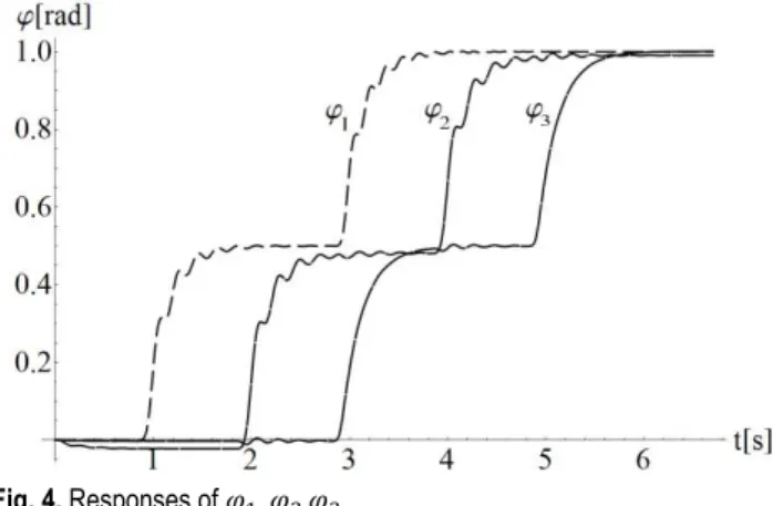
This section discusses the results of a simulation of closed-loop equations including a robot model with PD controllers (Fig. 4). The collected data will then be used in the identification algorithm.
First, the pre-determined signal was defined: [,<,=,>]. The signal was assumed to be a properly delayed step function (each arm with a different delay) passing through an additional low-pass filter with a boundary frequency Ω= 0.025 [rad/s]. The filtering was responsible for limiting the signal spectrum.
Fig. 4. Responses of , ,
The responses are not satisfactory from the point of view of regulation. The aim of the study was to generate signals to be used in the identification process. It is advisable that the pre-determined signals and the controller parameters be carefully selected so that the signals provide sufficient information about the object dynamics.
5. IDENTIFICATION WITHOUT MEASUREMENT NOISE Let us recall that the robot mass and arm length are the un-known parameters denoted as = [ , , , ", ", ", 23<, 23=, 23>]. The method used for the parameter iden-tification is represented graphically in Fig. 1. It is assumed that the measurement data concerning the trajectories of the generalized variables and the necessary input signals are available. The estimate of the input signals, ̂I, is determined basing on the current estimates of the object parameters = [ J, J, J, "K, "K, "K, 23<, 23=, 23>]. These equations have the same struc-ture as Eq. (23); yet, the unknown parameters , are replaced by the estimates , the generalized variables are replaced by varia-bles filtered through a low-pass filter, and their derivatives (which are not measured) are replaced by their estimates obtained by using relevant differentiating filters. Let us assume that the boundary frequency of the differentiating filters is: Ω= 0.2 [rad/s]. The identification requires determining the estimates of the parameters responsible for the quality factor minimization.
∫
− = T f f dt T J 0 2 ) ˆ ( 1 ) ˆ (θ τ τ , (24)where I is an input signal filtered with a low-pass filter.
The identification procedure is commenced for the following initial values: = [99.8, 151.7, 49.9, 0.49, 1.01, 0.75, 22.95, 22.95, 23.05]. The final values of the parameters are determined after 52 iterations of the minimization algorithm. The estimates = [76.616, 150.133, 49.9456, 0.57938, 1.0003, 0.700715, 23.0012, 22.9996, 23.0002] slightly depart from the real values of the parameters, = [100, 150, 50, 0.5, 1, 0.7, 23, 23, 23]. 6. IDENTIFICATION AND MEASUREMENT NOISE
In this point we will examine how far the elaborated filters eliminate the measurement and quantization noise (Mocak and other 2007; Rabiner and Gold 1975). We will also examine the influence of the measurement and quantization noise on the result of identification process with the use of finite elements differentia-tion method and elaborated filters.
The signal processing theory comprises activities aimed on selection of substantial information on the examined phenomena and elimination of redundant information. It is commonly known that the measured signals contain components resulting from the disturbances. In our case the quantization noise value is connect-ed directly with the number of bits of the n-bit A/D converter (Ly-ons 1999; Pintelon and Schoukens 1990).
Using the same identification method and elaborated filters following parameters have been obtained for the noisy signal (n=16) = [91.7605, 149.478, 50.8972, 0.516604, 0.9963, 0.691788, 23.0015, 22.9962, 23.0002], (n=14)
θ
ˆ=[11.4876, 153.601, 48.2456, -1.66054, 1.00276, 0.715608, 22.9934, 22.9787, 23.0018] .Using the finite elements method following parameters have been obtained for the noisy signal (n=16) = [2.62172*10^7, -2.31916*10^6, 530190.0, -0.0000152889, -0.000337396, 0.000112932, 15.3375, 14.4677, 22.5499].
Comparing the obtained results we can state that the differen-tial filters eliminate the measurement noise in a major degree and the parameters determined in the identification process are close to the actual ones. Traditional differentiation does not ensure noise elimination and the identified parameters differ significantly from the actual ones.
Using the elaborated filters in identification methods we obtain well determined parameters in case of quantization on the level of 16-bit cards.
7. CONCLUSIONS
In contrast to the conventional output error method, which in-volves comparing and estimating input signals, the input error method is considerably faster. The identification procedure does not require solving a series of differential equations in each itera-tion of the algorithm minimizing the quality factor.
It should be noted that the spectrum of the pre-determined signals is limited. In spite of the fact that the robot system is a non-linear system, the following relationship is obtained for the filtered signals: ̂I≅ I if = . As the slight differences are due to the system non-linearity and quantization errors, the equation can be solved approximately.
Elaborated differential filters have low-pass character. This feature enables removing of high-frequency components of the
signal, for example the noise. Differential filters ensure determin-ing of appropriate derivatives of signal with errors far more less than simple differentiation methods, what plays particularly im-portant role in the identification process. In various calculations which have been performed, proper operation of the method for more complicated mechanical systems and for systems of greater number of identified parameters has been stated.
REFERENCES
1. Cedro L., Janecki D. (2009), Differential filters and the identification of a manipulator using Mathematica software, XXXIV. Seminar ASR
'2009 Instruments and Control, Ostrava, ISBN 978-80-248-1953-2.
2. Cedro L., Janecki D. (2011), Model parameter indentification with nonlinear parameterization applied to a manipulator model,
Monographic series of publications-Computer science in the age
of XXI century, ISBN 978-83-7789-006-6, ISBN 978-83-7351-324-2.
3. Janecki D., Cedro L. (2007), Differential Filters With Application To System Identification, 7th European Conference of Young Research and Science Workers in Transport and Telecommunications
TRANSCOM 2007, śilina, Slovakia, p. 115.
4. Kowal J. (2004), Fundamentals of control engineering. Vol. II, UWND, Kraków.
5. Lyons R. G.(1999), An introduction to digital signal processing
(in Polish), WKiŁ, Warsaw.
6. Mocak J., Janiga I. I, Rievaj M., Bustin D. (2007), The Use of Fractional Differentiation or Integration for Signal Improvement,
Measurement Science Review, Volume 7, Section 1, No. 5.
7. Pintelon R., Schoukens J. (1990), Real-Time Integration and Differentiation of Analog Signals by Means of Digital Filtering, IEEE
Transactions on Instrumentation and Measurement. Vol. 39. No. 6.
8. Rabiner L. R. and Gold B. (1975), Theory and Application of Digital