Using Variational Methods
Sune Høgild Keller
The Image Group, Department of Computer Science
Faculty of Science, University of Copenhagen
Preface
This constitutes Sune Høgild Keller’s PhD thesis. The thesis is submitted at the Department of Computer Science (DIKU), Faculty of Science, University of Copenhagen in partial fulfillment of the requirements for the degree of doctor of philosophy.
This thesis was successfully defended on December 3, 2007. The evaluation committee was: Professor Gerard de Haan (Technical University Eindhoven and Philips Research), PhD Senior Researcher David Tschumperl´e (GREYC Lab, Caen, France) and Associate Professor Jon Sporring (DIKU, University of Copenhagen).
The first part of this work has been carried out at The Image Group, IT University of Copenhagen (ITU) in the period September 2004 to December 2006. The remaining work has been done at the Image Group, Department of Computer Science, Faculty of Science, University of Copenhagen in the period January 2007 to September 2007. All work has been supervised by Professor Mads Nielsen who is currently affiliated with the same group as me and director of Nordic Bioscience Imaging (NBI) a division of Nordic Bioscience A/S, Herlev, Denmark. Co-supervision has been done by Senior Researcher Fran¸cois Bern-hard Lauze of NBI (until December 2006 Assistant Professor with the Image Group at ITU).
It was the parallel between holes in interlaced video and holes in old films that gave birth to this PhD project. I was annoyed by the pour image quality on a standard interlaced tv-sets and Mads Nielsen and Fran¸cois Lauze were looking for new problems to tackle with variational methods. Thus the idea for the master thesis of Sune Høgild Keller [57] was borne. Then followed a patent application (US [66] and PCT [67]) on the idea of using energy minimization and variational methods for video upscaling in general and a grant making this PhD thesis possible.
Author Contact Information
Telephone: +45 26 79 09 79 Email: [email protected]
Home page: image.diku.dk/sunebio
c
Acknowledgements
So many people have helped me get to where I am today, but only a few have been mentioned here. I have a wonderful family and great friends, to whom I count almost all my colleagues: That’s how it goes when one has been lucky enough to work in both the former Image Group at ITU and in the Image Group at DIKU. To all of you, mentioned here or not, thanks!
Mads Nielsen provided me with the tools of how to fight the annoyance bad viewing experiences in my home cinema – sunebio. You were a great coach both professionally and mentally: You reach for the stars and I try to tag along. Thanks for a great skiing trip to Colorado!
Fran¸cois Lauze, you are French with a big fatFand your trademark ’double-wrues’. We didn’t always see eye to eye on how things should be done, but I believe it strengthened our joint work. You brought the math back into my life in the best of ways and you supervised me way beyond all requirements, mon ami.
Jenny, my ITU office buddy for two years at ITU, thank you for a great friendship and many shared experiences in the life of PhD students, heja Sverige. Thanks also to Rabia who gave me first class company while Jenny was away and to Aditya, David and Lars S. for doing the same at DIKU.
Kim Steenstrup Pedersen, you gave great support when I did it ’my way’ scientifically. Grumse, you told me how to keep Fran¸cois and Mads on a short leash. Marco who always listened when I needed to bitch or just talk, I think you are the colleague/friend with whom I shared the most good times – and beers. Thanks for the hill hike in Hofgeismar. Marleen, I really appreciate your friendship and professional advice – and how you made it crystal clear to me how good life as a PhD is in Copenhagen – at least compared to the Netherlands. Eugenio, you tried to charm the ladies old and young but you also charmed this guy into a great friendship. And I could go on about the rest of you: Eva, Anne, Ole, Erik, Lars C.-H., Michael, Jakob, Arjen, Arish, Pieter, Corn´e, Nanna, Pechin, Lauge and Vladlena. To Peter Jo, the rest of the ’old’ DIKU Image Group and Stig, thanks for making me feel welcome to DIKU.
Outside our own little duck pond here in Copenhagen, thanks to Sarang Joshi and Steve Pizer and his wife Lynn for given me a feel of the university life at UNC Chapel Hill. To the Saarbr¨ucken guys, Joachim, Andres and Martin for great discussions in Copenhagen and in scale spaces. And talking about scale spaces, thanks for sharing thoughts on science and PhD life to the Eindhoven gang, Bart, Erik, Bram, Frans and Evgeniya.
Then there are those who do not play with images. Camilla Torp-Smith, Lotte Møller, Gitte Hornstrup Dahl, Camilla Jørgensen and Marianne Henrik-sen, you all survive daily contact with us crazy scientist, thank you all for great help and advice.
My Family. My mother who has always been there for me, my sometimes annoying kid sister, I love you. My grandfather Ingolf who has taught through setting an example, how to keep my feet firmly planted on the ground, my late grandmother Ellen Marie who always paid me for my grades good or bad, my late uncle Gerwin for making me interested in technology and science and my father who did the same posthumously. Martin, Steffen, Helle, Gerda, Tom, Sofie and the rest of you.
Whenever I went flat on the batteries, I have always been able to go and reload in Krampam˚ala, paradise on earth in deep forests of Sweden. Thanks for many great times Gitte, Benny, Lasse, Thea, Susanne, Claus, Astrid and Christine.
Finally the biggest thanks of all to Bente, my wonderful fianc´ee, who has made the vast majority of my days the last seven years a perfect balance between a professionally fulfilling work life and a wonderful private life. Without you this dissertation would not have been, I dedicate it to you – det her er til dig, tak!
Abstract
In this thesis we do image sequence upscaling using variational methods. We have developed, implemented and tested the three main elements of the upscal-ing part of a video processor usupscal-ing variational methods plus a non-variational preprocessing method detecting the scan format of the input video. The three upscalings needed are deinterlacing (DI), which is creating the never recorded every other line in interlaced video, video super resolution (VSR), which is increasing the spatial resolution of each frame in the video throughput, and temporal super resolution (TSR), which changes the frame rate of a sequence by creating fully new frames at the correct temporal positions.
Our variational upscaling methods have been derived from a Bayesian infer-ence framework for image sequinfer-ence restoration and enhancement. The frame-work dictates simultaneous computation of the flow and intensities of the re-paired and/or enhanced output sequences. The framework was first suggested for image sequence inpainting in [65].
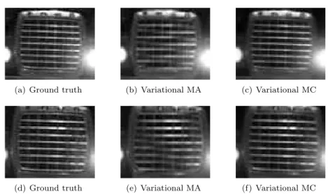
From the framework we derive a motion adaptive (MA) deinterlacer and a motion compensated (MC) deinterlacer and test them together with a selection of known deinterlacers. To illustrate the need for MC deinterlacing the inter-lacing problem is introduced. It cannot be solved by MA deinterlacers or any simpler deinterlacers but only by MC deinterlacers. The major hurdle in doing MC deinterlacing is reliable optical flow computations on interlaced video. We discuss a number of strategies for computing optical flows on interlaced video hoping to shed some light on this problem. We produce results on real world video data with our variational MC deinterlacer that even in many difficult cases are indistinguishable from the ground truth.
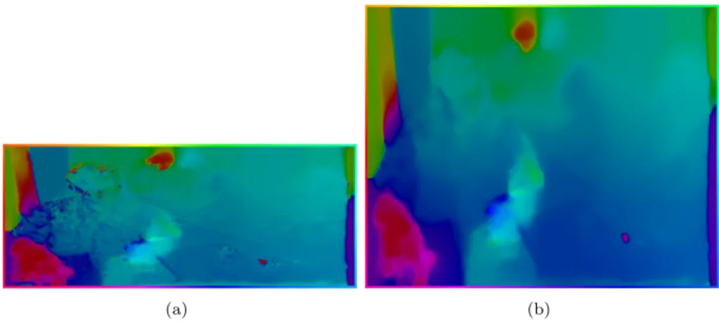
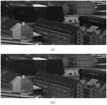
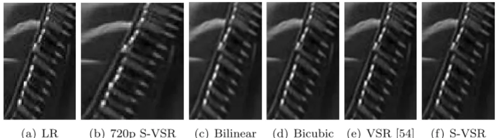
Producing high image quality on high definition (HD) displays when showing standard definition (SD) material is a problem of upscaling frame resolutions from low resolution (LR) to high resolution (HR) and is as such a super resolu-tion (SR) problem, or as we prefer: Video super resolution(VSR). In technology available today the problem is typically solved using simple spatial interpola-tion. Using motion compensated methods instead will allow for information transport along the optical flow trajectories of the video and increase the level of detail and sharpness in the high resolution output. We present a variational motion compensated VSR method derived from our Bayesian framework that simultaneously computes the desired high resolution video and a high resolution flow field to increase accuracy of the temporal information transport. Creating super resolution flows has to our knowledge not been done before. Most ad-vanced SR methods found in literature cannot be applied to general video with arbitrary scene content and/or arbitrary optical flows as it is possible with our simultaneous VSR method, which also allows for arbitrary discrete magnifica-tion factors. We show in test that our variamagnifica-tional simultaneous VSR algorithm outperforms other SR methods applicable to our general video problem, and we also attempt to break the limits of super resolution [2] in our experiments by increasing the frame resolution eight times in both height and width (8x8 VSR). Temporal super resolution (TSR), the ability to convert video from one frame rate to another is a key functionality in a modern video processing systems. A different and often higher frame rate than what is recorded is desired for high frame rate displays, for video/film format conversion, or for super slow-motion.
We present a novel motion compensated TSR algorithm using variational meth-ods for both optical flow calculations and the actual new frame interpolation as naturally derived from our Bayesian framework. The flow and intensities are calculated simultaneously in a multiresolution setting. We discuss what output quality is desired from a TSR algorithm. A major problem in watching video on large and bright displays is that the motion of high contrast edges often seem jerky. We test an implementation of our algorithm focussing on getting the motion of high contrast edges to seem smooth and natural by doubling the frame rate, thus reestablishing the effect of motion pictures.
We introduce an algorithm – commonly known as a film mode detector – for separating progressive source video from interlaced source video. Due to interlacing artifacts in the presence of motion, a difference in isophote curvature can be measured and a threshold for effective classification can be set. This can be used in a video upscaling to ensure high quality output as one can determine if deinterlacing is necessary or not.
Finally we discus the remaining unsolved problems in variational upscaling (hopefully) subject to future development. The most essential is realtime im-plementations of our algorithms, which from our assessment are doable with today’s technology.
List of Publications
Peer-Reviewed Conference Papers
• Sune Høgild Keller, Fran¸cois Lauze and Mads Nielsen, Motion Compen-sated Video Super Resolution, Scale Space and Variational Methods in Computer Vision, SSVM 2007 Proceedings, F. Sgallari, A. Murli and N. Paragios, editors, LNCS 4485, pages 801-812, Berlin, Springer, 2007.
• Sune Høgild Keller, Fran¸cois Lauze and Mads Nielsen, Variational Mo-tion Compensated Deinterlacing, 3rd Workshop on Statistical Methods in Multi-Image and Video Processing (SMVP), 9th ECCV Workshop Pro-ceedings, 2006.
• Sune Høgild Keller, Kim S. Pedersen and Fran¸cois Lauze, Detecting In-terlaced or Progressive Source of Video, Proceedings of the 2005 IEEE Seventh Workshop on Multimedia Signal Processing, 2005.
• Sune Høgild Keller, Fran¸cois Lauze and Mads Nielsen,A Total Variation Motion Adaptive Deinterlacing Scheme, Scale Space and PDE Methods in Computer Vision, 5th International Conference, Scale-Space 2005, Pro-ceedings, R. Kimmel, N. Sochen and J. Weickert, editors, LNCS 3459, pages 408-419, Berlin, Springer, 2005.
Patents
• Fran¸cois Lauze, Sune Høgild Keller and Mads Nielsen, A Method of Adding Information to a Frame or a Field in a Video Sequence, PCT Patent Application WO-A-2006/035072 (PCT/EP2005/054957), Sept. 30, 2005.
• Fran¸cois Lauze, Sune Høgild Keller and Mads Nielsen, A Method of Adding Information to a Frame or a Field in a Video Sequence, U.S. Patent Application US 11/239697, Sept. 30, 2005.
Technical Report
• Sune Høgild Keller, Fran¸cois Lauze and Mads Nielsen,Variational Dein-terlacing, IT University Technical Report Series, TR-2006-90, ISBN 87-7949-134-0, 2006.
Preface i Acknowledgements ii Abstract iv List of Publications vi 1 Introduction 1 1.1 The Challenge . . . 1 1.2 Motivation . . . 1
1.3 Organization of this Dissertation and How to Read It . . . 2
2 Background 4 2.1 Technical Overview . . . 4
2.2 Human Vision and the Displaying of Image Sequences . . . 5
2.2.1 Basic Properties of the Human Visual System . . . 6
2.2.2 Meeting the Requirements of the HVS in Technology . . . 8
2.2.3 Good and Bad Human Vision . . . 10
2.3 Quality Assessment: Objective vs. Subjective Measures . . . 10
2.4 Color Video Processing . . . 12
2.5 Optical Flow . . . 13
2.5.1 Temporal Information and Motion Compensation . . . 13
2.5.2 Motion and Optical Flow . . . 13
2.5.3 Variational Optical Flow . . . 15
2.6 Variational Upscaling Framework . . . 17
2.6.1 Bayesian Inference . . . 18
2.6.2 Variational Formulation . . . 20
3 Deinterlacing 22 3.1 Introduction . . . 22
3.2 Background and Related Work . . . 25
3.2.1 Simple Deinterlacing Techniques . . . 26
3.2.2 Motion Adaptive Deinterlacing . . . 26
3.2.3 Motion Compensated Deinterlacing . . . 28
3.2.4 Variational Deinterlacing . . . 29
3.2.5 Optical Flow Estimation in Interlaced Video . . . 30
3.3 Theory and Algorithms . . . 32
3.3.1 Variational Framework . . . 32
3.3.2 Selecting the Terms of the Energy . . . 34
3.3.3 Variational Motion Adaptive Deinterlacing . . . 34
3.3.4 Variational Motion Compensated Deinterlacing . . . 36
3.3.5 Numerics and Solvers . . . 39
3.3.6 Iterative Schemes . . . 42
3.3.7 Simultaneousness . . . 42
3.4 Experiments . . . 43
3.4.1 Quality Measurements . . . 43
3.4.2 Test Material and Online Video Results . . . 44
3.4.3 Initialization Tests . . . 44
3.4.4 Objective vs. Subjective Results . . . 44
3.4.5 Best Motion Adaptive Deinterlacer . . . 47
3.4.6 Variational Motion Compensated Deinterlacing Results . 48 3.5 Conclusion and Future Work . . . 53
4 Video Super Resolution 55 4.1 Introduction . . . 55
4.2 Background . . . 58
4.2.1 The Super Resolution Problem . . . 58
4.2.2 Related Work on Super Resolution . . . 58
4.2.3 The Foundation of Our Method and Related Work on Variational Methods . . . 60
4.2.4 Modelling the Point Spread Function . . . 61
4.3 Variational Video Super Resolution . . . 62
4.3.1 Bayesian Framework and Motion Compensated Image Se-quence Upscaling and Restoration . . . 62
4.3.2 From MAP to Variational Energy Minimization . . . 63
4.3.3 Variational Video Super Resolution and Optical Flow . . 64
4.3.4 Simultaneous Optimization of High Resolution Flows and Intensities . . . 66
4.3.5 The Super Resolution Constraint . . . 67
4.3.6 Minimizing Algorithm . . . 69
4.3.7 Discretizations . . . 71
4.4 Experiments . . . 74
4.4.1 The Importance of the Super Resolution Constraint . . . 75
4.4.2 Subjective and Objective Evaluation . . . 75
4.4.3 Test Material . . . 76
4.4.4 Parameters . . . 76
4.4.5 Running Times . . . 77
4.4.6 Online Material and Correct Viewing of Results . . . 78
4.4.7 2x2 and SD to 720p Results . . . 78
4.4.8 Down and Up Again: Objective Results . . . 83
4.4.9 Attempting to Break the Limits of Super Resolution . . . 85
4.5 Improved Video Super Resolution . . . 88
5 Temporal Super Resolution 89
5.1 Introduction . . . 89
5.2 Background . . . 91
5.2.1 Problem Analysis: Frame Rate Requirements . . . 91
5.2.2 Blur Acceptance in Human Vision . . . 93
5.2.3 Strategies of Creating New Frames . . . 94
5.2.4 Simultaneous Flow and Intensity Calculations . . . 95
5.2.5 Worst and Best Case: Frame Doubling . . . 96
5.2.6 Super Slow-motion . . . 96
5.2.7 Other Work . . . 97
5.2.8 Benchmarking in Testing . . . 99
5.3 Theory and Algorithm . . . 100
5.3.1 Bayesian Inference and Variational Framework . . . 100
5.3.2 Variational Temporal Super Resolution . . . 101
5.3.3 Gradient Constancy Assumption on the Flow . . . 103
5.3.4 Temporal Super Resolution Is not Inpainting . . . 104
5.3.5 Motion Blur . . . 104
5.3.6 Algorithm for Frame Doubling . . . 105
5.4 Experiments . . . 107
5.4.1 Test Material . . . 107
5.4.2 Parameters . . . 108
5.4.3 Other Methods in Test . . . 109
5.4.4 Evaluation Strategy . . . 110
5.4.5 Frame Doubling Results . . . 110
5.4.6 Objective Evaluation of Frame Doubling Results . . . 115
5.5 Discussion . . . 118
5.5.1 Improving Variational Optical Flow in Motion Compen-sated Upscaling . . . 118
5.5.2 Pointers to Generic Variational Frame Rate Conversion . 121 5.6 Conclusion . . . 122
6 Detecting Interlaced or Progressive Source of Video 123 6.1 Introduction . . . 123
6.2 Theory . . . 124
6.2.1 The Difference Between Interlaced and Progressive . . . . 124
6.2.2 The Measurement – Isophote Curvature . . . 124
6.2.3 Measuring the Statistical Difference . . . 125
6.2.4 Edges . . . 125
6.2.5 Two Approaches to a Solution . . . 125
6.2.6 Comparing the Two Approaches . . . 126
6.3 Other Work . . . 126
6.4 Results . . . 127
6.4.1 Initial Testing . . . 127
6.4.2 Method One – Comparison withP . . . 128
6.4.3 Method Two – The Zigzag Solution . . . 128
6.5 Conclusion . . . 131
7 Summary and Future Work 132
7.1 Summary of Contributions . . . 132
7.2 Possible Future Developments . . . 134
7.2.1 The Modelling Problem: Priors and Data Terms . . . 135
7.2.2 Improving Flow Quality . . . 136
7.2.3 Speedups . . . 136
7.2.4 Towards an Integrated Variational Upscaling System . . . 138 7.2.5 Streamed Video Processing: Temporal Sliding Windows . 139
Appendix 142
A Large Size Video Super Resolution Figures 142
Introduction
1.1
The Challenge
The purpose of this PhD project has been to develop the elements needed for the upscaling part of a video processor using variational methods. The three types of needed upscalings are deinterlacing (DI), which is creating the never recorded lines in interlaced video, also known as interlaced to progressive conversion, video super resolution (VSR), which is increasing the spatial resolution of each frame in the video throughput, and temporal super resolution (TSR), which changes the frame rate of a sequence by creating fully new frames at the temporal positions where they are needed.
De-noising, image reconstruction and inpainting are some of the problems earlier tackled with success using variational methods. From the work done by Lauze in [64] we had the platform of doing variational based inpainting, and to put it simple, the job was no longer to repair pixels but to create new ones. Holes in images, whether it is the result of a damage to a film strip or lines not recorded in an interlaced video signal, are in a general sense the same, just holes. But as this work will show there is a is great deal more to doing upscaling than just applying an inpainting algorithm to the problem. When actually solving the problems it becomes clear that the three types of upscalings, DI, VSR and TSR are three quite different problems, making variational DI, VSR and TSR three challenging problems.
1.2
Motivation
Today’s video upscalers do not produce outputs of a quality good enough to please the human observers, and thus improved deinterlacers, frame rate con-verters (TSR) and spatial upscalers (VSR) are sought for in both broadcast-ing, film/tv production and home consumer products. Variational methods, although still only being an emerging technology, have already proven their worth in inpainting (see [64]) and thus it seemed obvious to us that variational methods would give high quality results if applied to the problem of video up-scaling.
prob-lem had only been attacked from an electronic engineering point of view and variational methods had never been applied to the problem. Along with the work of Tschumperl´e and Besserer in [102] (using 2D spatial structure tensors) we were the first to introduce variational approaches to the field of deinterlac-ing. Bayesian formulations, energy minimizations and total variation was not unknown to the field of super resolution (SR), but our ideas of a motion com-pensated approach with no limitations on the flow, and an algorithm producing simultaneously a) a high resolution sequence and b) a corresponding high reso-lution optical flow, are new. And the integration in our variational framework is also new. When it comes to temporal super resolution, motion compensated methods are the only way to get reasonable results, but mostly block matching flow estimation and simple temporal interpolation are used. Thus the simulta-neous calculation of both intensities and flows using variational methods is new. All in all the basics of a full research project was there, and work on this PhD thesis was started.
The general idea of variational, energy minimizing video upscaling given in the following chapter is also what is covered by the US and PCT patent applications [66] and [67]. It is our hope to see our algorithms implemented and used in ’real world’ video processing systems in the (near) future. This system could be placed in the editing room of a film/tv production company, at a broadcasting company doing HDTV transmissions or in a private home incorporated in video playback devices, displays, high end stand alone video processors like Faroudja’s DVP-1010 (see Chapter 3) or other electronic media devices.
Our focus throughout the process of doing this work has been to lift the bar on what can be achieved in terms of output image quality from video upscalers. The most likely reasons why variational methods have never been tried in up-scaling before, are that they are considered too computationally expensive and are relatively unknown in the field of electronic engineering. But the fast growth in the performance/price ratio of field-programmable arrays (FPGAs) and other multiprocessor technologies along with the work of Andres Bruhn and others (see e.g. [11]) on realtime variational optical flow computations on standard PCs, have assured us that realtime variational video upscaling is within reach at a reasonable price even today.
1.3
Organization of this Dissertation and How to
Read It
The basic idea of this project to build the elements of an upscaling video proces-sor is reflected in the organization of this thesis as the four main chapter each represents an element.
• In Chapter 2, before going into details with each element, we present the background of our work: We look at human vision, basic technical details and the general idea of building an inference machine, the philosophy and method leading to a model of image sequence enhancement and recon-struction in general and a video upscaling solution in particular.
vari-ational motion adaptive (MA) deinterlacing in the master thesis [57] of Sune Høgild Keller is presented along with the work on it successor, vari-ational motion compensated (MC) deinterlacing. The chapter is intended for future journal publication in IEEE Transactions on Image Processing. Earlier versions of the work has been published in [55] and [53].
• Chapter 4 is on video super resolution (VSR) and also intended for journal publication. Initial work on variational video super resolution not produc-ing high resolution flows along with the high resolution intensity sequences was published in [54].
• Chapter 5 is on temporal super resolution (TSR). Although intended for journal publication, it is written in integrated chapter form, requiring prior reading of Chapter 2 to get the in-depth picture. Chapter 3 and Chapter 4 can be read independently of any other chapters, but readers will benefit from also reading Chapter 2.
• In Chapter 6 we present a scan format detector separating interlaced video from progressive video by measuring curvature statistics. The scan format detection is a crucial preprocessing step in upscaling, determining whether or not to deinterlace a given input. This work was earlier published in [56]. The ordering of the Chapters 3–5 above suggests our basic idea of how to cascade the three types of upscaling in a video processor. If the input is progressive to begin with but packed in an interlaced broadcast signal as is the case with for instance cinematic movies, one needs to bypass the deinterlacing simply just rejoining the separated frames. Determining whether the signal is progressive or interlaced is not straightforward and that is where the method of Chapter 6 comes in. Although format detection is a preprocessing step, we have placed in the back as it is the smallest of the four contributions represented by the Chapters 3–6, and the chapters 3–5 relates directly to the general idea presented in Chapter 2 and each other. Since Chapters 3, 4 and 6 are written in the form of stand alone publications, they can be read individually. Reading the full thesis some redundance will inevitable occur, mainly in the theoretical parts of the chapters. To the reader less experienced with variational methods this might serve as a help to understand the field.
Finally, in Chapter 7 we summarize and look ahead, discussing how the work presented in this thesis can possibly be used and improved in the future, for instance we look at how to organize and integrate the three upscalings steps deinterlacing, video super resolution and temporal super resolution.
Background
In this chapter we will go through the most important parts of the foundation of knowledge on which our work stands. We will start by giving an overview of the technical details in video and broadcasting today in Section 2.1, then we look at human vision in Section 2.2 as it is the sense we wish to optimally stimulate with our results. In Section 2.3 we then look at how to measure the quality of our work by it deviation from a ground truth or by how pleasing it is to the human visual system. Section 2.4 is on color versus grey scale video upscaling and Section 2.5 discuss work on variational optical flow, which is integrated into our variational video upscaling framework presented in Section 2.6.
2.1
Technical Overview
Since this section is dense with facts upon facts, to keep it fairly readable, we have not stated references for each and every small piece of information. As main sources of information we have used [4], [70], [82], [97], [98] and [107], and we only give the main, necessary information leaving out the details not needed explicitly in this thesis.
In Europe the dominating broadcasting standards are PAL (Phase Alter-nating Line) and SECAM (S´equentiel couleur `a m´emoire) which in their ana-log forms have an apparent resolution of 576 horizontal lines of video. They both transmit 50 interlaced fields per second, each field containing 288 lines of video, alternatingly the even numbered or the odd numbered horizontal lines (illustration given in Figure 3.1(b) in Chapter 3 on deinterlacing). The name interlacing comes from the fact that the transmission order is even-odd-even etc. and as such the fields seems interleaved or interlaced. The North American and Japanese standard is called NTSC after the National Television System Committee and is likewise interlaced but with 480 apparent horizontal lines of video and 60 fields per second.1 In their digital forms used on storage media like
DVD Video and in digital broadcast, the resolutions are vertical by horizontal, PAL and SECAM: 576×720 pixels, and NTSC: 480×640.
1Nominally 60 Hz/100.1%≈59.94 to avoid interference with the 60 Hz power source it was
set to match originally. In the same way PAL and SECAM match 50 Hz AC power sources, but due to the different color systems used, only NTSC had serious interference problem. Still NTSC is popularly know to be short for Never The Same Color.
Most flat panel screens (Plasma, LCD plus some emerging new technolo-gies), projectors (DLP, LCD etc.) and classic ’deep’ PC monitors (cathode ray tube, CRT) are progressive, meaning they need deinterlacing – interlaced to progressive conversion – to be able to show interlaced PAL, SECAM and NTSC broadcasts or video. Furthermore most displays are of a higher spatial and/or temporal resolution and thus requiring video super resolution and/or temporal super resolution. The old standard definition (SD) formats are slowly being replaced by high definition (HD) formats, the dominating ones being 720p (720×1280 progressive, 24, 25, 30 or 50 fps) and 1080i (1080×1920 interlaced, 50 or 60 fps) or 1080p (1080×1920 progressive, 24, 25 or 30 fps). These formats are used in high definition television (HDTV) broadcasts and on the new digital video disc media HD DVD and Blu-ray disc.
PAL, SECAM and NTSC use the academy screen aspect ratio with a 4:3 = 1.33:1 frame width to height aspect ratio, whereas the HD formats are widescreen with a 16:9 aspect ratio. The academy format was the preferred film aspect ratio until the 1950s recommended originally by the American Academy of Motion Picture Art and Sciences, thus the name. As television took over the format, motion pictures gradually switched to widescreen formats, e.g. cine-mascope. The HD pixels in widescreen are 1:1 in size, but with use of 1.422:1 pixels PAL also exists as an SD widescreen format, which is used for most cine-matic moves on DVD.2 The pixel squeeze used is similar to the format squeeze
obtained when recording films with an anamorphic lens to get e.g. 2.35:1 cine-mascope and thus denoted anamorphic widescreen.
Telecine is a process scanning recordings from film to video and even though they are displayed at 50 or 60 interlaced fields per second, they are recorded progressively at 24 frames per second (fps). Converting progressive source video back from interlaced is called a pulldown – 3:2 for NTSC and 2:2 for PAL and 30 fps film recordings (many US tv shows, e.g. sitcoms like Friends). Thus deinterlacing only denotes the process of actually creating extra lines in interlaced to progressive conversion.
All these facts on standards given above arise not only from technical and physical issues and limitations. The values and characteristics as for instance frame rates, are often fixed at their given values to accommodate properties of the human visual system (HVS), and interlacing was also employed to (ab)use properties of the HVS. To optimize the viewing experience, the THX norm (www.thx.com) was defined based on the minimum requirements needed to give a ’good’ movie experience. Thus sound and video equipment and movie theaters upholding this norm gets THX certified as a sign of high technical quality.
2.2
Human Vision and the Displaying of Image
Sequences
The reason why we are at all interested in doing upscaling is to enhance the viewing experience of human beings. There is no doubt that visual processing takes up a lot of the capacity of the human brain. Better visual inputs will give
2This pixel ratio is most often given as 1:1.422. There seems to be no general agreement
on whether to use height:width or width:height when giving aspect, pixel, screen and frame ratios or sizes, but we will try to stick to using height:width in accordance with the rows, columns notation used for 2D matrices.
Figure 2.1: The human eye. Figure from [73].
two improvements. First, the better the input provided the less resources are spend processing it, which makes the viewing experience more relaxing. Second, the more natural the input appears, the less it will annoy the viewer. And that is what we are after.
Visually pleasing a human being can be done on several levels. On the high-est level it is a quhigh-estion of psychology, does a person like certain colors more than other colors, does she prefer football over fashion shows, horror movies over comedies etc. All lower level vision serves to aid higher level vision. In providing quality inputs for the lower level vision, technology help film direc-tors, tv producers etc. get their message through, e.g. by making sure the viewer sees colors the right way, that the image sequences displayed are sharp and detailed, that there is no annoying artifacts brought forth by bad record-ing, transmission, storage, coding etc. We do not want to change the artistic (or commercial) message presented by the sender, but we wants to make sure it reaches its human receiver as undistorted as possible, providing the lower level vision with optimal input. Unless references otherwise, the sources of any infor-mation given in the following subsections of this section (2.2) are the excellent book on human sensation and perception by Matlin and Foley [73], and to a lesser extent the book [43] by Gonzalez and Woods on digital image processing. Certain technical details mentioned are given in the references mention at the beginning of Section 2.1.
2.2.1
Basic Properties of the Human Visual System
The lower level part of the human visual system (HVS) consist of the eye, a vi-sual pathway and (parts of) the vivi-sual cortex in the brain. A schematic drawing of the eye is shown in Figure 2.1. Light is projected through the lens and the cornea, ensuring (in the healthy eye) the information carried by the light reaches the retina covering the back of the inside of the eye. The retina is covered by photoreceptors called rods and cones. The rods gives us the ability to see when
there is very little light, but only provides grey scale information. The widely used RGB color model is based over how the cones operate: There are three kinds of cones each covering parts of the visual light spectrum giving us color vision when there is an abundance of light available. The photoreceptors are connected vertically through bipolar cells to ganglion cells, each of the ganglions collecting the input from a number of photoreceptors forming a receptive field. It is the size of these receptive fields that crudely put decides the resolution of the eye and the HVS. But the density of receptive fields vary on the retina and already in the horizontal interconnection of photoreceptors and receptive fields through amacrine and horizontal cells complexity is added to the processing of the visual stimuli and the same goes for it passage through the visual pathway also doing some processing of the data. This illustrates how complex human vision is and explains why measuring and deciding on the properties of the HVS is not straightforward.
It is however a given fact that the stimuli of the receptive fields are treated in the visual cortex. On a higher level complex objects are recognized, but very interestingly the less complex processing in the visual cortex responds to edges, producing different signals according to the orientation and strength of the given edge. This makes edges a primary cue in vision. When there is no edges in the light signal projected onto the receptive fields in the retina, no signal is transmitted from the edge processing cells in the visual cortex connected to this receptive field. Thus we have to fill data from around edges into any smooth area where there is no edges present to give stimuli. Thus the variational image model total variation modelling images as smooth regions separated by edges mimics the lower level human vision rather well.
We have so far been concerned with the spatial processing of the HVS, but the time dimension also plays a role. A uniformly colored input (no edges seen in it) covering the full visual field will over time fade to a medium gray as there is no changes in the input to the eye over time and the receptive fields will just transmit a ’standby’ or ’null’ signal. It is changes in light the cells register and to keep the input from fading the eye makes small rapid movements all the time. When there are no edges no changes occur and thus the fading described above occurs, but only after a while (when both the memory stored and the filling-in effect described further above will fade out). A bit more important to our work is the fact that the eye to a certain extent is able to track and give the HVS a fixed and detailed view of moving scenes and objects. Another very interesting fact and the reason we have motion pictures is that the eye can be fooled to see motion where there is really none. Stroboscopic movement, e.g. created by flashing a light briefly at one location of the retina and shortly after flashing another light at another location will make the viewer perceive it as just one light moving in a straight line from one position to the other. The same sensation of movement is obtained with most rapidly changing patterns, e.g. still images only shown briefly to create motion pictures.
The eye is generally very sensitive to changes in stimuli (mostly induced by movement in the scene viewed) especially away from the center of focus on the retina (the fovea). The size of the area changing is also important to the response of the eye, the larger the area of change, the larger the sensitivity. The sensitivity to temporal changes in stimuli is called flicker sensitivity in the field of image sequence display.
Figure 2.2: The projection of an on-screen image onto the retina. α is the vertical viewing angle dependant of the screen heighthand the viewing distance
d. The same relations are found for the horizontal (and diagonal) directions. The resolution of the screen ultimately set the limit of the maximal viewing angle possible.
2.2.2
Meeting the Requirements of the HVS in Technology
The many characteristics of the lower level HVS given above have been impor-tant in fixing the specifications of the video and broadcast standards described in section 2.1. Here we will discuss some the connections from HVS to technical specifications and requirements.
First, the spatial resolution of a discrete (digital) image stimuli has to meet the resolution of the HVS. The resolution of a screen is critical to how close viewers can be placed to the screen without spotting pixels instead of what appears to be a continuous image. The viewing distance and the size of the screen decides the viewing angle and the size of the projection of the image onto the retina. A sketch of this projection is given in Figure 2.2.
We know that a) pixels are square and receptive fields mostly circular, b) receptive fields are unevenly distributed on the retina and of different sizes, c) the visual processing and perception of details more complex than just defining the size of receptive fields, and d) the properties of the stimuli (brightness, color etc.) and viewing conditions affect the viewing experience. Thus the minimum required resolution of an image display at a given viewing angle has to fixed empirically. The THX norm requires horizontal viewing angles of at least 25◦ to probably ensure engulfment in the visual experience, keeping the viewer
focused on the on-screen story and nothing else. Since degrees are not that easy to measure in the living room, the equivalent minimum viewing distance required is more widely used. On an standard PAL 576i tv-set the minimum viewing distance is six times the height of the screen. With the higher vertical resolution obtained by switching to progressive, a 576p screen should be viewed at distance of at least 4.3 times the height [108]. Thus deinterlacing increases the engulfment at a given screen size if it is done right (that is, deinterlacing without creation of visually annoying artifacts). Increasing the spatial resolution (VSR) will enable increased viewing angle and also lift the viewing experience if done right. The viewing distances given here and in [108] for other formats as well are not fixed as many factors decide the minimum and optimal viewing distances, but the viewing distance given serve as a frame of reference.
We have now established that increased spatial resolution is beneficial thus justifying the need for deinterlacing and video super resolution but also the
temporal resolution is important.
The ability of the eye to induce apparent motion when exposed to rapidly changing patterns is used to make thephi-effectoccur: Frame recordings (stills) of moving objects are shown in succession at a rate high enough to makes the motion depicted seem fluent. This is motion pictures. In early film recordings 16 fps was considered enough to create the phi-effect, but as technology evolved the film recording frame rate was since increased to 24 fps, which is the rate still used today. The rapid change of images needed to create motion pictures can (depending on the screen size and brightness etc.) be sensed by the eye as flickering, thus often requiring the frames to be updated faster than what is required to obtain the phi-effect. That is one of the major reasons why the PAL, SECAM and NTSC standards have field rates of 50 and 60 Hz.3
The area dependency of the flicker sensitivity in the eye described at the end of Section 2.2.1 is why interlacing exists. Each line can be updated at half the rate at which the full screen is updated without the eye sensing it – the area of a single line is too small to make it flicker in the eye in spite of it low refresh rate. But as screens grew larger and brighter (in living rooms not growing at the same speed) the flicker of single lines became apparent. With that a need of breaking the limits set by the SD television formats appeared. Before HDTV was introduced, PAL tv-sets with doubled field rates (100 Hz) where developed in a successful (but time limited) attempt to improve quality without changing the broadcasting standard.
The viewing angle dictated by the viewing distance (fairly static in most homes) and screen size is the major reason why higher refresh rates are needed, but also the screen type (CRT, LCD, plasma, film/DLP/LCD projector), screen brightness, image content and the general viewing conditions (lighting condi-tions in the room mainly) puts requirements on the refresh rate. Higher refresh rates can however be obtained by just redisplaying the same frame, which works fine on e.g. computer monitors as they mainly show stationary content.
In movie theaters with 24 fps recorded progressive on film (similarly on LCD screens) one can just let the current image be displayed constantly for 1/24 of a second as it will not flicker. The same goes in principle with e.g. LCD screens as they do not suffer from the same problem as CRT screens (and to some extent plasma screens): The image on screen will fade over (very short) time on a CRT and thus needs refreshing in order not to flicker. Projection of the same progressive frame or image for a longer time onto the retina – even just for 1/24 second in moderns cinemas – will make it appear to be a still image and thus give a sense an abrupt transition to the next frame and destroy the illusion of fluent motions otherwise obtained by the phi-effect. Therefore a shutter (a rotating disc which is semi hole, semi impenetrable to light) in the projector will give short blackouts once or twice during the display of a single frame, increasing the frame rate to 48 or 72 fps. The same need exist on LCD screen displaying video. Still, with only 24 fps recorded, high contrast edges in motion will sometimes appear as moving jerky thereby breaking the illusion of motion pictures. This failure to uphold the phi-effect also goes for video versions of film recordings and HD recordings at lower frame rate. Thus the need for increased temporal resolution is there.
3The values were beyond what was needed with early tv sets under normal viewing
con-ditions, but the values were fixed at these specific values to correspond with the frequency of the electrical AC power supply to simplify the engineering of tv sets as mentioned earlier.
2.2.3
Good and Bad Human Vision
As mentioned above the retina photo receptor resolution is not decisive when it comes to the limit of detail perception in the HVS. Recent research by Rucci
et al. [87] has confirmed what was long suspected: The rapid eye movements do not only serve the purpose of keeping visual stimuli from fading over time, it is also used to increase perceived resolution by integrating the low resolution input of the retina over time. This is human vision at its best.
The eye is able to track motion in an observed scene to a certain limit, and when this limit is crossed only motion blurred input is received on the retina. But in some cases the HVS fools its owner by deciding to classify some (motion blurred) input as sharp even though it is only registered in a blurred version on the retina, [15] and [74]. This could be seen as a counterpoint to the case of good vision described just above. In the space between the two cases we need to provide sharp an detailed video input at a reasonable computational cost. The challenge will be to produce as sharp and detailed video as possible and keep it free of any artifacts. We must try to remove artifacts present in the input and not introduce new ones in the upscaling process. In the next section we will discuss how to measure the quality of our upscaling results.
2.3
Quality Assessment: Objective vs. Subjective
Measures
”Do you like fermented beans?” Ask a person this and many will not know what fermented beans are and among those who know, mostly Japanese people will answer yes as it is a traditional Japanese dish. Taste, emotions, feelings, inheritance and environment; humans are formed and driven by many factors hard to measure as objectively as a number, we are individual beings with subjective opinions and tastes. When it comes to vision there might be similar measurable neural responses in lower level vision to a given visual input, but we can unfortunately not use these lower level patterns to predict how each individual judge or psychologically interpret the visual stimuli leading to this specific neural pattern. The human psyche and the brain as such are not (yet) mapped to a degree enabling quantification of it, and we are anyway highly subjective in our judging of visual – and other – inputs.
Using statistics on a larger number of subjective evaluations done by hu-man observers can of course give some average answers on e.g. the quality of a given video enhancement method. But statistically significant answers require a large test panel and a standardized test setup like the ITU4
recommenda-tion for subjective quality assessment of video in [50]. The Danish producer of audiovisual consumer electronics Bang & Olufsen has its own setup using both layman and expert panels [100] and the same goes for Philips in the same line of business as described in [4]. These large scale subjective evaluation setups are so time and resource consuming that they are often not used when presenting new video processing methods. The alternatives are either smaller subjective test panels consisting of the authors and maybe some colleagues, or (simple) objective measures – or often both. Typically results are compared to results
obtained by existing methods, simple or advanced, to show the qualities of the new method presented – in the good cases the visual differences are very clear and thus the advantages of the new methods clearly shown.
Objective measures give clear cut differences between results obtained with different methods and leaves no room for interpretation, but are also often very far from giving a true picture of how the results would be evaluated by a large group of subjective viewers. Objective measures require a ground truth for comparison and thus we artificially need to create the degraded low resolution video by removing (scan) lines, downsampling frames, or removing frames. This will of course only serve as a simulation of real ’degraded’ data (e.g. video recorded with an interlaced camera) and thus devaluate the use of objective measures. Exceptions from the requirements of a ground truth sequence are the MTI and MSEi measures for deinterlacing evaluation given by Bellers and
de Haan in [4], but the measures then depend on the optical flow computed on the sequence. The two most widely used objective measures are: Mean square error (MSE) and peak signal to noise ratio (PSNR). We have used objective evaluation with varying success. For assessment of deinterlacing (Chapter 3) we show how the MSE does not correspond with the subjective evaluation, whereas it corresponds perfectly in video super resolution evaluation (Chapter 4) and temporal super resolution evaluation (Chapter 4). For the case of deinterlacing a study of quality assessment carried out by Zhao and de Haan in [109] compares PSNR with an 18 person subjective evaluation finding statistically significant correlation between the two. This study can along with ours be considered limited cases, as the data sets are small (in [109] only five test sequences are used and the test data is also subject to some postprocessing before the subjective evaluation is carried out).
In our opinion objective evaluation gives a hint of what to expect from a sub-jective evaluation, but should never be used on its own, this goes also for more advanced objective measures that claim to model the HVS closely. 36 objective measures are put to the test by Kanters in [51] to evaluate image reconstruc-tion, and it is”...concluded that it is almost impossible to find an objective error measure that correctly resembles the human observer results.” ([51], Chapter 4, p. 76.) We agree on this and are of the opinion that in limited cases (small data set or certain tasks, e.g. video super resolution) some objective measures might actually agree quite well with the subjective evaluation, an opinion that it is also uttered by Kanters in [51] and Nadenauet al. in [77]. In the latter Nadenauet al. summarizes the results of a larger test of subjective (following [50]) and objective video quality evaluation by the Video Quality Experts Group (VQEG) [106]. The correlation in quality ratings between subjective evaluations conducted at different labs is 0.9 - 0.95 while the best objective measures only have correlations of 0.8 - 0.85. In [84] Puttensteinet al. have tested 20 objective quality measures in evaluating noise reduction in video, and found none of them to correlate very well with the subjective evaluations conducted as well.
In the conclusion of [84] Puttensteinet al. writes: ”Even a combination of objective measures only approximates the subjective assessment of the quality of noise reduction algorithms with a descriptive power as low as 59%.” In the conclusion of the report by the Video Quality Experts Group [106] it is stated that the VQEG does not recommend the addition of any objective measure to the ITU Recommendations on video quality assessment. Furthermore it is stated that no objective measure is able to replace subjective evaluation, a conclusion
we had also drawn before knowing of this report.
The objective measure used most widely for assessment of accuracy in op-tical flow calculations, the average angular error (AAE) suffers from the same problems as the objective image quality assessment measures and can only be used on artificial sequences due to the lack of a ground truth optical flows on real world sequences.
2.4
Color Video Processing
All inputs and results given in this thesis are 8-bit luminance channel video. There are several reasons why we have not produced color video results. First, and least important is that in many publications color printing is not an option or rather expensive and thus it is customary to present gray scale results only. Secondly, extension to full RGB or YCrCb is straightforward as all channels
can be processed independently using the same code as applied to just the luminance channel. More advanced vectorized version of our algorithm could be devised (e.g. following the directions given in[103]) which should give better coherence in geometrical structures between the three channels and thus better results. This leads us to the third reason why we do luminance processing only: Advanced vectorized color processing will most likely not be beneficial on video in general. Analog video is broadcasted and stored using half of the total bandwidth available for the luminance channel, sharing the other half between the two color channels [70]. This has two reasons, first, using YCrCb
and not RGB made it easy to add color information to the black and white broadcasting signals so that people were not forced to buy new color tv sets and the broadcasters not forced to broadcast both in color and black and white. At the same time the subsampling of the color channels made room for more broadcast channels. Secondly, the HVS is less sensitive to information (on edges) given in the color channels than information given in the luminance channel. The color compression by subsampling w.r.t. to the full frame resolution has also found its way into digital video and broadcast where MPEG-2 used on DVDs and its HD successors (MPEG-4/H.264) all subsample the color channels when applied in practice on video. The term 4:2:2 describes the sampling ratios of the YCrCb signal and along with 4:1:1 (or 4:2:0, see [107] for details) this
factor two subsampling in one or two dimensions are the commonly used color formats.
Therefore it is obvious to just apply simpler methods for the color channels in deinterlacing. As described in Chapter 3, throwing the full variational algorithm at the color channels is a complete waste of resources. For temporal super resolution where fully new frames are created it will of course be necessary to fully process the color channels, but since the resolution of each color channel is 50 or 25% of that of the luminance channel and the flow will be almost directly reusable as the channels are highly correlated, the computational overhead will be small. For video super resolution simple interpolation could be used on the color channels as long as the magnification factors are not to large, but when the full algorithm needs to be applied, the flow can again be reused.
2.5
Optical Flow
In this section we will give a short introduction to the importance of knowing how an image sequence changes from one frame to the next, how we find the optical flow of the image sequence. Focus will be on how we can use optical flow computations to improve upscaling by doing motion compensation (MC).
2.5.1
Temporal Information and Motion Compensation
It should be clear by now, that temporal information is of high value in video processing. In the 2D spatial plane of an image or video frame, we have in each point access to neighboring information, helping us to improve processing. The information could be knowledge of edges, how strong are they and what are their orientations, helping us to preserve and maybe even enhance the edges when processing the frame. There is an abundance of information available in image sequences due to the (relatively) dense temporal information sampling. If there is no or only very small motion (less than one pixel in size in the digital/discrete image sequence grid) the relevant temporal information correlated to the pixel currently being processed is easily found. In case of larger motion we need to follow the trajectory of the motion to find the relevant temporal information: We do motion compensation, which requires an estimation of the motion first.
Motion compensation is a cornerstone of all our upscalings and in any image sequence with motion it is crucial to now the flow if one wants to optimize the output quality. But there is a price to pay for the gain in quality: Estimating reliable and precise motion is a complex task.
2.5.2
Motion and Optical Flow
The physical world is 3+1D (3D space and 1D time). In a projection of the world into 2+1D as done when recording image sequences (2D spatial image frames and time) information will be lost, and thus we can only do an estimation of the real, physical 3D motion. The intensities (or in many cases, color) and positions projected onto the 2D frame plane is all the information we have available when estimating the motion in image sequence analysis and processing – but also as human viewers of film, video and television. The apparent motion perceived when viewing or analyzing 2+1D image sequences is in the computer vision literature calledoptical flow.5 Optical flow does in some cases differ from the
true projected 2D motion, the textbook example being the zero optical flow in a projection of a rotating, uniformly colored sphere, the true projected 2D motion being the rotation. An illustration of this example is given in Figure 2.3. The optical flow maps the changes from one frame into the next, which is what we would like to compute when doing motion compensated video upscaling. Any knowledge of the geometrically true 2D motion or for that matter the physically true 3D motion, will not improve the upscaling and thus the data we transmit to the eye via the display as it is still just an optical 2D projection. In other fields of computer vision, e.g. robot navigation, true 3D motion reconstruction is of great importance.
5We will use the terms optical flow computation/calculation/estimation and motion
es-timation interchangeably from here on, as we do estimate the motion when computing the optical flow.
000000 000000 000000 000000 000000 000000 000000 000000 000000 000000 000000 000000 000000 000000 000000 000000 111111 111111 111111 111111 111111 111111 111111 111111 111111 111111 111111 111111 111111 111111 111111 111111 00000000 00000000 00000000 00000000 00000000 00000000 00000000 00000000 00000000 00000000 00000000 00000000 00000000 00000000 00000000 00000000 11111111 11111111 11111111 11111111 11111111 11111111 11111111 11111111 11111111 11111111 11111111 11111111 11111111 11111111 11111111 11111111
3D object Image plane
Figure 2.3: A uniformly colored sphere rotating around any of its own axes on the left and its projection onto the image plane on the right. Any 2D rota-tion (speed and axis) can be projected but the optical flow either computed or perceived will be zero unless additional information is provided. Figure from [64].
The foundation of optical flow calculation is the assumption that one can find information recorded in one frame in the next frame as well even if objects in the recorded scene moves around. We are looking for a displaced frame difference (DFD). It is typically assumed that the information we are looking for is (pattern of) intensities that do not change from frame to frame. Thus the DFD is also known as the brightness (or grey level) constancy assumption (BCA) and is
u(x+~v, t+ 1)−u(x, t) = 0 (2.1) whereu=u(x, t) is the 2+1D image sequence withx= (x, y) being the spatial coordinates and t the time dimension. The optical flow we are looking for is
~v= (v1, v2) where (v1, v2) are the (x, y)-coordinates of the flow from frametto
framet+ 1 assuming a distance of 1 between neighboring frames.
The intensities (or colors) cannot be expected to stay the same from frame to frame: A red ball is also red in the next frame no matter if it moves or not, but not if the lighting of the scene changes. The gradient constancy assumption (GCA)
∇u(x+~v, t+ 1)− ∇u(x, t) = 0 (2.2) which assumes the image gradient ∇u stays constant, helps to cope with the instability of the BCA under changing lighting conditions. The gradient of the edge between white an black patches of a football stays (close to) constant even if the light on the ball changes.6
6Gradients are the almost salient measure of edges in images and as we know from
Sec-tion 2.2, edges is a key cue to the lower level vision. Thus computing optical flows with good gradient/edge mapping will be a help in doing good motion compensation.
Figure 2.4: The aperture problem in optical flow computation. Two edges and corner moves from frame t to frame t+ 1. In Aperture 1 we cannot uniquely identify the correct flow, but in Aperture 2 we have enough (local) information to uniquely determine the correct flow.
When computing optical flows one would like to get it very detailed and thus use a small aperture in which we define the flow for each part of a frame. The aperture is often a small block (e.g. 8x8 pixels) or single pixels in discrete settings. But when we use a small aperture, we do not always get all the information we need to calculate the flow correctly. The general problem of only having very local knowledge of what is going on is called the aperture problem. Say we have a line moving, then any point on the line in frametcould go to any point on the line in the next framet+1 as illustrated with ’Aperture 1’ in Figure 2.4. Say we extend our aperture to include a corner at the end of the line, then in the corner point we have spatial gradient in two direction and can determine the exact flow for the whole line as with ’Aperture 2’ in Figure 2.4. The second fundamental problem in computing optical flows is the occlusion problem. When an object moves it covers (occludes) and uncovers (disoccludes) background or other objects behind it in the scene. Since we are looking for similarities between frame we have a problem when information is only present in one of the frames. A solution to the problem when one needs the flow to do motion compensated video processing, is to look for information along the flow both backwards and forwards in time.
In the next section we will look at how we solve the aperture problem and handle the occlusion when using variational methods to compute optical flows.
2.5.3
Variational Optical Flow
Variational methods for optical flow calculations are among the most accurate in existence as found in the major survey by Bruhn et al. in [12] and they fit perfectly into our variational framework presented later in this chapter. A very detailed work on variational optical flow is the PhD thesis by Bruhn [13].
All three of our upscalings (DI, VSR and TSR) are motion compensated thus they need an optical flow field to be operational.7 This complicates matter
as typical implementations of variational optical flow methods can be compu-tationally heavy. However, being able to draw on temporal information from neighboring frames is a major gain and will provide improved quality (e.g. shown for the case of inpainting in [64] by Lauze). Returning to the computational
7We also present a motion adaptive deinterlacing algorithm but our focus is on the motion
complexity of variational optical flow methods, it is possible to run them in re-altime. In [11] Bruhnet al. presents an implementation of a linear, variational flow algorithm that produces dense web-cam resolution (18 frames per second (fps), 252×316 spatial resolution) flows in realtime on a standard PC. The nonlinear methods we used are (a lot) more complex and even SD video (PAL, 25 fps, 576×720) requires more resources, but with dedicated hardware and the right amount of parallel processors it should not be impossible as we will discuss in Chapter 7 of this thesis.
Fitting any variational optical flow methods into our framework given later in Section 2.6, is straightforward. Practically all variational flow methods from the early method of Horn and Schunck in [48] to the so far most accurate method by Brox et al. presented in [9] consists of two terms. The first is a data fidelity term defining the temporal correspondence from frame to frame and is derived from the brightness and gradient constancy assumptions in (2.1) and (2.2). The second term is a prior on the flow telling us about the expected local correlation between neighboring flow values. In short the prior models the fact that local clusters of pixels will have the same or very similar motion as they will represent just one object with (relatively) uniform motion due to the physical rigidity of the world. It is more probable that neighboring pixels will have the same flow than have very different flow. The prior is also the key to solving the aperture problem, although we really do not care where on the line in Aperture 1 in Figure 2.4 we get our information from when using the flow for motion compensation. Still, the prior term imposes a necessary regularization on the optical flow computation not provided by the data term.
In the pioneer work by Horn and Schunck [48] the data term is the classical optical flow constraint (OFC),
~v· ∇u+ut= 0 (2.3)
where ∇u= (∂u/∂x, ∂u∂y)T and u
t is the derivative ofu w.r.t. time.
Equa-tion (2.3) is the differential and linearized version of the brightness constancy assumption in (2.1). The OFC can also be written
~v· ∇u+ut=V~T∇3u=£V~u= 0
where ∇3 is the spatiotemporal gradient of u, V~ = (~vT,1)T and £V~u denotes
the OFC as the Lie-derivative ofualong the flowV~ (see e.g. [42]).
In [9] Brox et al. combines the BCA in the data term with the gradient constancy assumption, which in its linearized form is
£V~∇u= 0 (2.4)
theV~-directional derivative of the spatial image (frame) gradient.
Taking the classical approach to variational optical flow computations, the prior term is added to the BCA data term as the aperture problem is an ana-lytical derived consequence of having one equation (the BCA data term) with two unknowns, v1 and v2 of the flow vector ~v = (v1, v2). But still with the
GCA added to give us the extra equation, the regularization imposed by the prior (smoothness term) is important to get a dense flow field by pushing flow values into areas where salient image content is missing (e.g. along the line in
Aperture 1 of Figure 2.4. If the line from Aperture 1 to the corner in Aper-ture 2 is long, the aperAper-ture will be too small even with the prior added. The well-established solution to this problem is to first scale down the sequence and compute an initial guess of the flow at a coarser version of the image sequence. This is known as the multiresolution approach when it is done in several steps forming a pyramid of scales. Since the optical flow constraint and the linearized GCA are implemented as filter with only very local support, it will take many iterations to compute flows of high magnitude. Using multiresolution will also scale down the magnitude of the flow and thus also aid computation of high magnitude flows.
Between the landmark works by Horn and Schunck [48] and Brox et al.[9] many variations of variational optical flow have been suggested. For in-depth reading on variational optical flow we refer to the PhD theses by Bruhn [13] and Lauze [64]. We ended up mainly using the method of Brox et al. [9] as it is the most accurate method and had also been used successfully for motion compensated inpainting by Lauze and Nielsen [65].
The use of this method (and other variational approaches) on real world video has been relatively limited. When evaluating the quality of a method, the goal is to minimize the angular error to the ground truth flow, which only exist if the test sequence has been artificially generated like theYosemitesequence mostly used in optical flow benchmarking. Thus we conducted a tedious but also thorough test to optimize the settings in our implementation of the method from [9] (on both interlaced and progressive video) by visually judging the quality of the flow fields obtained using different parameter settings on real world data. The optimal parameter settings are the ones presented in each of the Chapters 3, 4 and 5 of this thesis.
2.6
Variational Upscaling Framework
Our upscaling problems are sampling problems. Deinterlacing and video super resolution are subsampling problems as the number of recorded spatial samples is too low compared to what we need. Temporal super resolution is in most cases also a subsampling problem, but can also be a case of upsampling. As we will make clear in Chapter 5 on temporal super resolution, creating fully new frames is a hard problem no matter whether you increase or decrease the frame rate of a sequence.
We will start our problem analysis using the sampling theory on the sub-sampling problem. In the recording process the 2+1D data projected from the real world has been sampled at frequencies lower than what we would like to display it at. The Nyquist-Shannon (sampling) theorem
Fmax≤ Fs
2
tells us to use a sampling frequencyFsat least twice as high as the highest
fre-quencyFmaxwe want to be able to sample from our signal. In video this decides
how fine details of the scene depicted we will be able to include. Frequencies higher thanFs/2 will be aliased if present in the signal and no (analog) low pass
The essential message we get from this analysis is that our upscaling prob-lems as they are subsampling probprob-lems by birth, are ill-posed. We will never be able to create what was never sampled, the sub-sampling process is an ir-reversible problem. Due to the presence of motion temporal super resolution is also an ill-posed problem when decreasing the frame rate. Spatiotemporal frequency analysis of the deinterlacing problem in the presence of motion has conducted by Bellers and de Haan in [4].
2.6.1
Bayesian Inference
To model image sequences, their optical flow and content and to impose some regularity to the ill-posedness we need an inference machine. The human viewer might be satisfied with many different solutions to our problems, but even if the human observer cannot see when or if the sampling process has been reversed, trying to go back as far as we can towards the analytically true solution is a good idea. We know it will be satisfactory for sure and where we cannot get close, the regularity will help us not stray to far in a wrong direction. Especially if the model applied for regularization lies close to how the human visual system itself imposes regularity and generally processes visual input. Exemplified the above problem view means that going towards how an standard definition signal would have looked recorded in high definition (HD) is a good idea when doing upscaling. Doing so we should impose regularity in our model to avoid creat-ing new artifacts (e.g. the rcreat-ingcreat-ing patterns often created by super resolution algorithms) that would annoy the viewer.
The inference machine we will use to define a framework for our upscaling problem of creating new data in an image sequence and impose some regular-ization on the ill-posedness of the problem is the Bayesian inference
p(a|b) =p(b|a)p(a)
p(b) (2.5)
where p(a|b) is the a posteriori, p(b|a) is the likelihood, p(a) the prior on (or simply the probability of)aandp(b) is the evidence ofb.
When it comes to the need of (re)creating information never sampled or missing due to a degradation of the image sequence data, de-noising, inpainting and upscaling are very similar problems. The similarity becomes even clearer when defining a joint framework of the problems using Bayes inference. Substi-tutingawith ua desired output image (de-noised, upscaled or inpainted) and
bwithu0 the input image (e.g. noisy, of low resolution or scratched), we get
p(u|u0) = p(u0|u)p(u)
p(u0) . (2.6)
To keep this example clear, we have started looking just at single images. The likelihood p(u0|u) is also known as the data (fidelity) term in variational
for-mulations as it tells us how the input relates to the output, e.g. how to place the existing lines of an interlaced signal in the deinterlaced, progressive output.
p(u) is the spatial prior on u, which decides what image content we allow in our images, how we model images. Maximizing the a posteriori, equal to maxi-mizing the right hand side in (2.6), optimizes the probability ofuknowingu0,
![Figure 2.1: The human eye. Figure from [73].](https://thumb-us.123doks.com/thumbv2/123dok_us/9960549.2891374/17.892.240.739.194.471/figure-the-human-eye-figure-from.webp)