Thesis for the degree of Licentiate of Engineering
Deep Learning Applications
for Autonomous Driving
LUCA CALTAGIRONE
Department of Mechanics and Maritime Sciences CHALMERS UNIVERSITY OF TECHNOLOGY
Deep Learning Applications for Autonomous Driving LUCA CALTAGIRONE
c
LUCA CALTAGIRONE, 2018
THESIS FOR LICENTIATE OF ENGINEERING no 2018:02
Department of Mechanics and Maritime Sciences Chalmers University of Technology
SE–412 96 G¨oteborg Sweden
Telephone: +46 (0)31–772 1000
Chalmers Reproservice G¨oteborg, Sweden 2018
Deep Learning Applications
for Autonomous Driving
Luca Caltagirone
Department of Mechanics and Maritime Sciences Chalmers University of Technology
Abstract
This thesis investigates the usefulness of deep learning methods for solving two important tasks in the field of driving automation: (i) Road detection, and (ii) driving path generation. Road detection was approached using two strategies: The first one considered a bird’s-eye view of the driving scene obtained from LIDAR data, whereas the second carried out camera-LIDAR fusion in the camera perspective. In both cases, road detection was performed using fully convolutional neural networks (FCNs). These two approaches were evaluated on the KITTI road benchmark and achieved state-of-the-art performance, with MaxF scores of 94.07% and 96.03%, respectively.
Driving path generation was accomplished with an FCN that integrated LIDAR top-views with GPS-IMU data and driving directions. This system was designed to simultaneously carry out perception and planning using as training data real driving sequences that were annotated automatically. By testing several combinations of input data, it was shown that the FCN having access to all the available sensors and the driving directions obtained the best overall accuracy with a MaxF score of 88.13%, about 4.7 percentage points better than the FCN that could use only LIDAR data.
Keywords: deep learning, computer vision, autonomous driving, robotic perception and planning, sensor fusion
Acknowledgements
I would first like to express gratitude to my supervisor Prof. Mattias Wahde for his faith in me and for his guidance in taking my academic career in the directions that I have.
My heartfelt thanks also go to my co-supervisor Prof. Lennart Svensson for his thoughtful advice and many stimulating discussions. I would like to thank Dr. Mauro Bellone for sharing his knowledge and for helping me keep my Italian alive.
I am very grateful to the PRELAT project for funding the work presented in this thesis and to Dr. Martin Sanfridson for keeping the project running. Last but not least, I wish to thank all my colleagues at VEAS for creating a very welcoming and friendly working environment.
List of included papers
This thesis consists of the following papers. References to the papers will be made using Roman numerals.
I. Caltagirone, L., Scheidegger, S., Svensson, L., and Wahde, M., Fast LIDAR-based Road Detection Using Fully Convolutional Neural Net-works. In: Proceedings of the 28th IEEE Intelligent Vehicles Sympo-sium, Los Angeles, CA, pp. 1019-1024, 2017.
II. Caltagirone, L., Bellone, M., Svensson, L., and Wahde, M., LIDAR-based Driving Path Generation Using Fully Convolutional Neural Net-works. In: Proceedings of the 20th IEEE International Conference on Intelligent Transportation Systems, Yokohama, Japan, pp. 573-578, 2017.
III. Caltagirone, L., Bellone, M., and Wahde, M., LIDAR-Camera Fusion for Road Detection using Fully Convolutional Neural Networks. Sub-mitted to Robotics and Autonomous Systems, January 2018.
Technical terms used in the thesis
Activation function, 4
Artificial neural network (ANN), 3 Artificial neuron, 3 Batch size, 11 Classification, 9 Context module, 23 Convolution, 7 Convolutional layer, 5
Convolutional neural network (CNN), 5
Cross fusion, 25
Deep neural network (DNN), 21 Dilated convolution, 23
Dilation factor, 23 Early fusion, 25 Encoder-decoder, 8
Exponential linear unit (ELU), 5 Feature map, 8
Fully connected network, 3
Fully convolutional neural network (FCN), 9 Hidden layer, 3 Hyperparameter, 8 Input layer, 3 Kernel, 7 Late fusion, 25 Max pooling, 8 Max unpooling, 9
Maximum F1-score (MaxF), 22 Output layer, 3
Pooling index, 9 Precision (PRE), 22 Recall (REC), 22 Receptive field, 5
Rectified linear unit (ReLU), 5 Regression, 9
Semantic segmentation, 10 Softmax function, 10
Stochastic gradient descent (SGD), 11 Stride, 7
Unit, 3 Weight, 4 Zero padding, 7
Table of Contents
1 Introduction and motivation 1
2 Convolutional neural networks 3
2.1 Artificial neural networks . . . 3
2.1.1 Artificial neuron . . . 4
2.2 Convolutional neural networks . . . 5
2.2.1 Convolutional layer . . . 5
2.2.2 Max pooling layer . . . 8
2.2.3 Encoder-decoder network . . . 8
2.3 Training and objective function . . . 9
2.3.1 Softmax function . . . 10
2.3.2 Cross-entropy loss and optimization . . . 10
3 Data set and preprocessing 13 3.1 Point cloud top-view representation . . . 13
3.2 GPS-IMU top-view representation . . . 14
3.2.1 IMU augmentation . . . 16
3.2.2 Driving intention . . . 18
3.3 Point cloud projection and upsampling . . . 18
4 Applications 21 4.1 Road detection . . . 21
4.1.1 LIDAR-only segmentation . . . 23
4.1.2 LIDAR-camera segmentation . . . 25
4.2 Driving path generation . . . 28 ix
x TABLE OF CONTENTS
5 Conclusion and future work 31
5.1 Conclusion . . . 31 5.2 Future work . . . 32
6 Summary of included papers 35
6.1 Paper I . . . 35 6.2 Paper II . . . 35 6.3 Paper III . . . 36
Bibliography 37
Chapter
1
Introduction and motivation
Every year about 1.3 million people die worldwide in road traffic accidents [27] and 20 to 50 million are injured or disabled. Road traffic accidents are currently the leading cause of death among young people aged 15 to 29 years. Besides human suffering, road traffic accidents also cause the loss of about 3% of global GDP [6]. According to the Tri-level study of the causes of traffic accidents [26], human factors were a probable cause in about 93% of the examined accidents. The above numbers clearly indicate that if human errors and deficiencies were removed from driving, there would be enormous savings both economically and in terms of human lives [2]. This consideration is one of the main motivating factors for the development of vehicles that drive autonomously, that is, vehicles that can understand the world and make decisions by themselves, without human input.
Driving a vehicle is quite a complex skill. Broadly speaking, it can be split into three main components: perception, planning, and control. Perception is the act of apprehending the environment in the immediate surroundings of the vehicle and it includes tasks such as recognizing whether there are other traffic participants and, if so, estimating their relative position and velocity, locating the road and its lanes and estimating the vehicle position within them, monitoring the vehicle state, and looking for traffic signs, traffic lights, and other relevant landmarks. Given this knowledge, a driver can plan the desired vehicle trajectory (planning) and then follow it by applying appropriate actions to the vehicle’s steering wheel, brakes, throttle, and gear shift (control).
The ultimate goal of driving automation is to develop computer systems 1
2 Chapter 1. Introduction and motivation that can carry out the previously described functions in all situations, effec-tively replacing the human driver. This is called level 5 automation, or full automation, according to the driving automation levels for on-road vehicles defined by SAE [25]. Many automotive and technology companies (e.g., Volvo Cars, Toyota, Google-Waymo, Apple), universities (e.g., Chalmers University of Technology, Oxford University, Stanford University), and startups (e.g., Otto, Drive.ai) are currently working towards this goal and much progress has been made in the past two decades. However, there are still many open problems to solve, in particular regarding the perception function in chal-lenging scenarios (e.g., rainy and snowy weather, nighttime, etc.).
Given that the transportation infrastructure has been tailored for human drivers who mainly rely on vision for sensing the environment, a natural choice is to equip autonomous vehicles with cameras in order for them to perceive the world. The information content of camera images is, however, strongly dependent upon the external lightning conditions and can be de-graded to a large degree in certain circumstances. It is therefore common to equip autonomous vehicles with additional sensors such as radars, sonars, and LIDARs that can provide a complementary or alternative view of the envi-ronment. For example, whereas cameras provide information about emitted or reflected light from surrounding objects (passive sensing), LIDARs gener-ate a sparse 3D representation of the scene by using their own emitted light (active sensing).
The information acquired by the sensors must then be processed us-ing computer algorithms that extract the information necessary to control the vehicle. Unfortunately, camera images and 3D point clouds are high-dimensional objects that are quite expensive to process. Only in recent years, with the advent of fast GPUs and novel machine learning techniques, has it become possible to accomplish that goal in real time and with portable com-puting devices.
As previously mentioned, autonomous driving is dependent on the con-certed action of many different functions. Furthermore, each function can be approached using a wide variety of algorithms. In this work, two tasks are investigated: (1) Road segmentation, and (2) driving path generation. Both were addressed using a family of machine learning algorithms known as deep learning [14]. These functionalities were developed and evaluated using the KITTI data set [10]. Finally, two main sensors have been considered, a monocular RGB camera and a multi-layer rotating LIDAR.
Chapter
2
Convolutional neural networks
2.1
Artificial neural networks
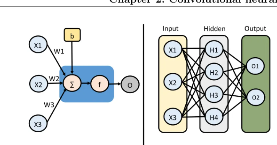
Artificial neural networks(ANNs) are a family of computing systems that are inspired by biological neural networks. The basic building block of all ANNs is the artificial neuron. Artificial neurons (or units) receive inputs from other neurons in the network and then generate their own output. The computation of the output as well as the connectivity among neurons depend on the specific application. In fact, many strategies have been developed since McCulloch and Pitts first proposed this type of computational model in 1943 [17]. This work focuses on multi-layer feedforward neural networks, that is, networks where the units are organized in multiple distinct layers, such that the information propagates only in one direction. The right panel of Fig. 2.1 shows an example of a feedforward ANN with three layers: (1) The leftmost layer is called the input layer and its nodes simply return the input data. (2) The inner layer processes the information coming from the input layer and its result is forwarded to the following layer. (3) The rightmost layer, or output layer, carries out further processing and generates the ANN’s final output. Layers that are placed between the input and output layers are called hidden layers. The ANN example just described is a fully connected network, that is, each unit in a given layer is connected to all the units in the previous and following layers. This connectivity is not efficient for working with high-dimensional inputs, such as images, because the number of connections becomes very large. Moreover, the fully connected architecture does not explicitly exploit the spatial structure of the information.
4 Chapter 2. Convolutional neural networks X1 X2 X3 W1 W2 W3 b O X1 X2 X3 H1 H2 H3 H4 O1 O2
Input Hidden Output
∑ f
Figure 2.1: (Left panel): A simple illustration of an artificial neuron receiving inputs from three units. The artificial neuron computes the sum of its inputs {xi}i=1,2,3 multiplied by their corresponding connection weights{wi}i=1,2,3, adds a bias termb, applies an activation function f, and then sends its output forward to other units. (Right panel) Illustration of a three-layer feedforward neural network. The information flows from the input to the output layer passing through one intermediate layer, called the hidden layer. The ANN is fully connected meaning that each unit in a given layer is connected to all the units in the preceding and following layer.
2.1.1
Artificial neuron
The output of an artificial neuron (see, for example, the left panel of Fig. 2.1) is computed by applying a function f, also known as an activation func-tion, to the weighted sum of all its K inputs plus a bias term b, that is:
o =f XK i=1 wixi+b , (2.1)
where the coefficientswirepresent the strength of the connections (orweights)
between the artificial neuron and its input units.
Over the years, many activation functions have been proposed, from the step function used in the perceptron [23] to the sigmoid logistic function. All of them, however, are nonlinear: This is a crucial requirement since otherwise, any number of layers could always be reduced to one, given that the composition of multiple linear transformations can be expressed as a single linear transformation. Nowadays, the most commonly used activation
2.2. Convolutional neural networks 5 function is the rectifier [14] that is defined as follows:
f(x) = max(0, x). (2.2)
A neuron that utilizes the above transfer function is called arectified linear unit (ReLU) [19]. Another popular activation function that has been shown to speed up learning and that is used in this work is theexponential linear unit (ELU) [5] :
f(x) =
(
x if x≥0
a(ex−1) otherwise where the parameter a is commonly set to one.
2.2
Convolutional neural networks
As mentioned in Sect. 2.1, fully connected neural networks are not efficient for processing high-dimensional inputs such as images. By studying the hu-man visual cortex, it was observed that individual neurons only have access to a small portion, called the receptive field, of the entire visual field [12]. Information is then aggregated by neurons that have overlapping receptive fields and neurons in deeper layers of the visual cortex. Biological consid-erations then suggest that local connectivity and hierarchical layers might be better suited for processing visual information. These observations were the inspiration for the development of theconvolutional layerwhich is the building block of convolutional neural networks (CNNs) [14].
2.2.1
Convolutional layer
In contrast to a fully connected layer, artificial neurons in a convolutional layer only have access to a limited region of the preceding layer, a region specified by their receptive field size. If this size is small, the number of connections is reduced significantly in comparison with a fully connected layer. Another important feature of convolutional layers is that the weights are shared among units which further decreases the number of parameters. The rationale behind this design choice is that discriminative features can be found anywhere in the visual field; a pattern of connectivity that detects vertical edges will likely be useful in the top right corner of an image just as much as in its bottom left corner.
6 Chapter 2. Convolutional neural networks R11 R12 R13 R14 R21 R22 R23 R24 R31 R32 R33 R34 R41 R42 R43 R44 B11 B12 B13 B14 B21 B22 B23 B24 B31 B32 B33 B34 B41 B42 B43 B44 K(R)11 K(R)12 K(R)13 K(R)21 K(R)22 K(R)23 K(R)31 K(R)32 K(R)33 ∑X=RGB (X11*K(X)11 + X12*K(X)12 + X13*K(X)13 + X21*K(X)21 + X22*K(X)22 + X23*K(X)23 + X31*K(X)31 + X32*K(X)32 + X33*K(X)33 ) ∑X=RGB (X12*K(X)11 + X13*K(X)12+ X14*K(X)13 + X22*K(X)21 + X23*K(X)22 + X24*K(X)23 + X32*K(X)31 + X33*K(X)32 + X34*K(X)33 ) ∑X=RGB (X21*K(X)11 + X22*K(X)12 + X23*K(X)13 + X31*K(X)21 + X32*K(X)22 + X33*K(X)23 + X41*K(X)31 + X42*K(X)32 + X43*K(X)33 ) ∑X=RGB (X22*K(X)11 + X23*K(X)12 + X24*K(X)13 + X32*K(X)21 + X33*K(X)22 + X34*K(X)23 + X42*K(X)31 + X43*K(X)32 + X44*K(X)33 ) K(G)11 K(G)12 K(G)13 K(G)21 K(G)22 K(G)23 K(G)31 K(G)32 K(G)33 K(B)11 K(B)12 K(B)13 K(B)21 K(B)22 K(B)23 K(B)31 K(B)32 K(B)33
Input 3x4x4
Kernel 3x3
G11 G12 G13 G14 G21 G22 G23 G24 G31 G32 G33 G34 G41 G42 G43 G44Output 2x2
R11 R12 R13 R14 R21 R22 R23 R24 R31 R32 R33 R34 R41 R42 R43 R44 B11 B12 B13 B14 B21 B22 B23 B24 B31 B32 B33 B34 B41 B42 B43 B44 Max (R11,R12,R21,R22) Max (R13,R14,R23,R24) Max (R31,R32,R41,R42) Max (R33,R34,R43,R44) Max Max Max MaxInput 3x4x4
Kernel 2x2
stride 2
G11 G12 G13 G14 G21 G22 G23 G24 G31 G32 G33 G34 G41 G42 G43 G44Output 3x2x2
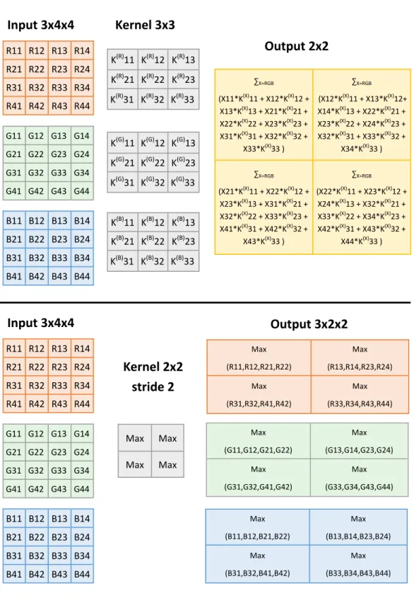
Max (G11,G12,G21,G22) Max (G13,G14,G23,G24) Max (G31,G32,G41,G42) Max (G33,G34,G43,G44) Max (B11,B12,B21,B22) Max (B13,B14,B23,B24) Max (B31,B32,B41,B42) Max (B33,B34,B43,B44)Figure 2.2: (Top panel) Illustration of the convolution operation carried out using a kernel of size 3×3 and stride 1. (Bottom panel) Max pooling operation performed using a filter of size 2×2 and stride 2.
2.2. Convolutional neural networks 7 A convolutional layer processes information structured as multidimen-sional arrays (henceforth: tensors). An RGB image, for example, can be represented as a 3D tensor of size D×H×W, where D denotes the depth (or number of channels, which in this case equals three), H is the height, and
W is the width. Given a kernelK of size F ×F and an input tensorI, the convolution operation is defined as follows:
O(i, j) = (I∗K)(i, j) = D X l=1 F X m=1 F X n=1 Il(i+m, j+n)Kl(m, n), (2.3)
The top panel of Fig. 2.2 illustrates this operation: given an input of size 3×4×4 and a kernel of size 3×3, an output of size 2×2 is produced by sliding the kernel window over the input tensor and applying the convolution operation. The stride of the convolution, denoted as S, controls how many cells the kernel should slide over each time it is moved. In the example above, the strideis set to one. Notice that only the spatial size of the kernel is specified, in this case F = 3; its depth is always constrained to be equal to the number of channels of the tensor it is applied to. As can be seen in Fig. 2.2, the spatial size of the output is smaller than the input. In general, the output size can be computed according to the following equation:
Wout =
(Win−F)
S + 1 (2.4)
Hout = (Hin−F)
S + 1 (2.5)
In some cases, it is desirable to control the spatial size of the output; a com-mon approach to achieve that is to pad the input with zeros before carrying out the convolution, a procedure known aszero padding. Letting P denote the amount of zero padding, Equations (2.5) and (2.4) then become:
Wout =
(Win−F + 2P)
S + 1 (2.6)
Hout = (Hin−F + 2P)
S + 1 (2.7)
Here, it is assumed that zero padding is applied symmetrically on both spatial dimensions; for example, P = 1 corresponds to adding two rows of zeros to the input, one at the top and one at the bottom, and two columns, one to
8 Chapter 2. Convolutional neural networks the left and one to the right. This procedure must be applied to each input channel.
The example shown in the top panel of Fig. 2.2 considers only one kernel which transforms the 3D input into a 2D tensor. In practice, however, a convolutional layer usually consists of many kernels and its output is also a 3D tensor. Each channel (i.e., 2D output obtained by applying one kernel) of the output tensor is called afeature map. To summarize, the output in channelzof a convolutional layer withZ feature maps is obtained as follows:
Oz(i, j) = (I ∗Kz)(i, j) = D X l=1 F X m=1 F X n=1 Il(i+m, j +n)Kzl(m, n) +bz, (2.8)
where now also the scalar bias term, bz, of feature map z and z∈(1, . . . , Z)
has been included.
2.2.2
Max pooling layer
In order to decrease the spatial size of the tensors processed with convolu-tional layers, it is common practice to insert in the network one or moremax poolinglayers. In this way, it is possible to reduce the memory requirements for training and running the CNN. Additionally, this operation provides par-tial translation invariance. A max pooling layer is entirely specified by its filter sizeF and its strideS. The bottom panel of Fig. 2.2 shows an example of the max pooling operation, considering a filter of size 2×2 and stride 2. The output tensor is obtained by sliding the max pooling filter across the input and by choosing the maximum value within the selected region; this operation is carried out on each feature map individually, so that the output will have the same depth as the input.
2.2.3
Encoder-decoder network
The previous sections presented some of the components that can be used when designing CNNs. It is easy to see that there are countless ways of selecting the layers’ hyperparameters (e.g., kernel size, stride, number of feature maps, etc.) and their mutual connectivity. This work focuses on one type of architecture known asencoder-decoder, an illustration of which is provided in Fig. 2.3. The key ideas of this architecture are (i) to decrease the spatial size of the input through a sequence of max pooling layers while
2.3. Training and objective function 9
Convolution 3x3, stride 1, zero-pad + ELU
Max pooling 2x2, stride 2 Max unpooling Softmax
W H D W H D W H D W H D W H N O U T P U T W/2 H/2 D
Conv 3x3, stride 1, zero-pad
I N P U T W/2 H/2 D*2 W/2 H/2 D*2 W/4 H/4 D*2 W/4 H/4 D*4 W/4 H/4 D*2 W/2 H/2 D*2 W/2 H/2 D*2 W/2 H/2 D Encoder Decoder
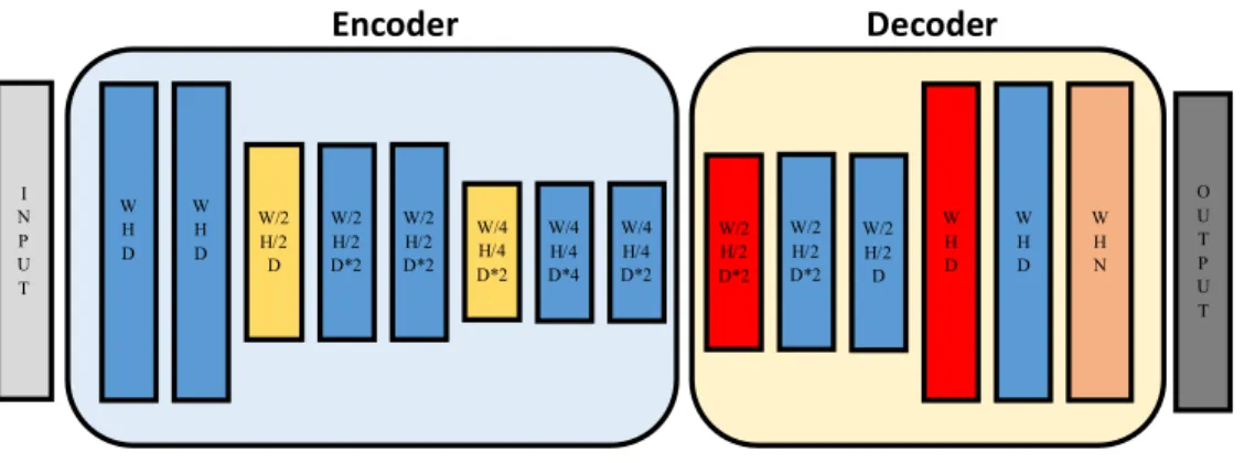
Figure 2.3: Encoder-decoder CNN. The encoder consist of a sequence of con-volutional and max pooling layers. The input spatial size is decreased after each pooling operation, thus reducing the memory requirements. At the same time, the number of trainable parameters is increased by doubling the number of feature maps in the convolutional layers. The decoder carries out further processing while also upsampling the spatial size of the input tensor. W is the input width, H is the input height, and D is the initial number of feature maps. N is the depth of the output tensor.
at the same time (ii) increasing the depth of the convolutional layers. With this strategy the memory requirements are reduced and the number of tun-able parameters is increased with each downsampling stage. The example in Fig. 2.3 shows a network with two downsampling and two upsampling stages. The max pooling layers also store the positions of the maximum values (pooling indices) in their input tensors. Those indices can then be used for carrying out the max unpooling operation in the decoding part of the network [1]. When a CNN, such as the encoder-decoder presented in this section, does not contain any fully connected layer (see Sect. 2.1), it is commonly referred to as a fully convolutional neural network (FCN).
2.3
Training and objective function
Machine learning can be used to solve many different tasks [11]. Two of the most common ones are classification and regression. In a classification
10 Chapter 2. Convolutional neural networks task, the algorithm should specify the class k ∈ 1, . . . , N that identifies a given input X. As an example, given an image, the task of the program might be to decide if there is a cat, or a dog, or a fox in it. Regression is similar to classification but, in this case, the output is a continuous variable instead of a discrete one. An example of regression is predicting the price of a house or a stock.
The work presented here is concerned with a task known as semantic segmentation, which can be seen as a generalization of the classification example described above. In this case, a program assigns to each pixel of a given image a probability distribution over the possible classes (e.g., road, car, pedestrian, etc.) to which the pixel could belong.
2.3.1
Softmax function
The softmax function, here denoted σ, is used to ensure that the out-put of an algorithm can be interpreted as a probability distribution. Each component of a vector z ∈RN is transformed as follows:
σ(z)i =
ezi
PN
j=1ezj
, i∈1, . . . , N (2.9)
It is easy to see that the components of the transformed vector are always positive and sum to one. For a semantic segmentation task, asoftmax layer is usually inserted after the last convolutional layer of a CNN. Its purpose is to apply the softmax function along the depth dimension at each spatial location in order to generate a probability distribution for each pixel.
2.3.2
Cross-entropy loss and optimization
Consider a classification task solved with an ANN parametrized by a vector of weightswand a training example (x, y), wherexdenotes the input andy rep-resents its corresponding ground truth class. Letfw(x) = f(x) = [p1, . . . , pN]
denote the ANN-predicted probability distribution over the possible classes. The cross-entropy error is then computed as follows:
H(x, y) =−log(f(x)y) = −log(py) (2.10)
The loss functionL used for tuning the ANN’s weights is commonly defined as the average cross-entropy error computed for the entire training set, that
2.3. Training and objective function 11 is: L(w) =− 1 M M X i=1 log(f(xi)yi) =− 1 M M X i=1 log(piyi) (2.11)
where M denotes the total number of training examples.
The minimization of the loss functionLis usually carried out using gradi-ent descgradi-ent and the backpropagation algorithm [24]. In practice, in order to reduce the computational burden, at each iteration the loss function is com-puted by considering only a randomly selected subset of the entire training set and the optimization algorithm is then known as stochastic gradient descent(SGD). The size of the subset is a hyperparameter called the batch size.
Chapter
3
Data set and preprocessing
This work makes use of the well-known KITTI Vision Benchmark Suite [10] which consists of many driving sequences logged over a period of several days in and around Karlsruhe, Germany, and includes urban, rural, and freeway scenarios. The data collection was carried out in day time and in fair weather conditions, using several sensors mounted on a Volkswagen Passat B6. Details about the setup can be found in [10]. The sensors relevant for this work are (i) an RGB camera (Point Grey Flea 2 FL2-14S3C-C), (ii) a LIDAR (Velodyne HDL-64E), and (iii) a GPS-IMU system (OXTS RT 3003). Fig. 3.1 shows a detailed illustration of the KITTI sensor platform1.
3.1
Point cloud top-view representation
In order to process a point cloud efficiently with a CNN, a preprocessing step is carried out for transforming it into a structured 3D tensor. The procedure consists of the following steps: (1) a 2D grid is specified in the x-y plane of the LIDAR coordinate system. Each grid cell has a size of L×L, where Lis set to 0.1 meters in this case. The region of space covered by the grid is set according to the specific problem under consideration: In Paper I, it covered
x∈[6,46] andy ∈[−10,10] meters; in Paper II, it covered for x∈[−30,30] and y∈[−30,30] meters. (2) Each of the 4D data points, which contains the position [x, y, z] and the reflectivity ρ, is then assigned to its corresponding
1http://www.cvlibs.net/datasets/kitti/setup.php
14 Chapter 3. Data set and preprocessing
Figure 3.1: Top view of the sensor platform used for data collection of the KITTI Vision Benchmark Suite [10]. The sensors relevant for this work are Cam 2, which is an RGB camera, the Velodyne laserscanner, and the GPS/IMU.
cell by projecting it onto the grid:
x y z ρ grid −−−−−→ projection u v z ρ (3.1)
whereu and v specify the column and row cell positions in the grid, respec-tively. (3) In each grid cell, several statistical measures are then computed: Number of points, mean reflectivity, as well as mean, standard deviation, minimum, and maximum height. (4) The complete point cloud top-view in-put is obtained by stacking together the 2D tensors corresponding to each statistical measures. Fig. 3.2 shows the top-view images obtained by applying the above procedure to an example from the KITTI road training set.
3.2
GPS-IMU top-view representation
This section describes how GPS-IMU information can be transformed into a spatial representation that is suitable for data fusion with the point cloud top-views described above, and that can be efficiently exploited by a CNN for pattern recognition.
3.2. GPS-IMU top-view representation 15
Figure 3.2: Each image encodes a specific statistic computed inside the grid cells using the procedure described in Sect. 3.1. (Top left) Maximum height. (Top center) Mean reflectivity. (Top right) Occupancy. (Bottom left) Elevation standard deviation. (Bottom center) Minimum height. (Bottom right) Number of points.
16 Chapter 3. Data set and preprocessing Consider a generic driving sequenceDconsisting ofN time steps. At each time step, the GPS-IMU system acquires the following information (only the relevant quantities are reported) about the vehicle state, (1) latitude, (2) longitude, (3) altitude, (4) roll angle, (5) pitch angle, and (6) heading. The data can then be summarized as a list of positions,{[x0i, yi0, zi0]T}Ni=1 and their corresponding pose matrices{Mi}Ni=1, with respect to a reference coordinate
system denoted by the superscript 0.
By selecting k as the current time step, it is then possible to define two sets of 3D points expressed in the current coordinate system, denoted by the superscript k, the future path Π+, and the past path Π−. For example, the vehicle relative future position at time stepk+2 can be obtained by applying the following transformation:
xkk+2 ykk+2 zkk+2 1 =M−k1Mk+2 0 0 0 1 . (3.2)
Each point in Π+ and Π− can then be projected onto the 2D grid specified in Sect. 3.1: xki yik zik −−−−−→grid projection ui vi . (3.3)
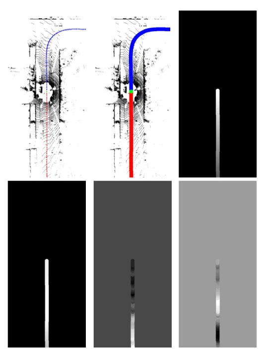
The top left panel of Fig. 3.3 shows an example of past and future paths rendered as disks in a point cloud top-view. The next step of the procedure is to join neighboring points in order to obtain a continuous curve (see the top middle panel of Fig. 3.3). In this case, the thickness of the driving paths is set to 18 pixels or 1.8 meters, which is the vehicle’s nominal width.
3.2.1
IMU augmentation
The future and past paths, so far, only contain occupancy information about whether the vehicle covered or will cover a certain grid cell (or pixel). The shape of the path already conveys useful knowledge that can, however, be augmented with additional information about the vehicle’s motion, that is, its forward speed, forward acceleration, and yaw rate. For each of those
3.2. GPS-IMU top-view representation 17
Figure 3.3: Illustration of the results generated using the procedure described in Sect. 3.2. (Top left) Discrete past and future paths represented by red and blue disks, respectively. The current position is drawn as a green disk. (Top middle) Continuous driving paths with thickness of 1.8 meters corresponding to the ve-hicle’s width. (Top right) Driving intention proximity encoding the approximate distance where a turning action should be taken. (Bottom) From left to right: Im-ages representing the vehicle’s forward speed, forward acceleration, and yaw rate. The grayscale intensities are proportional to the numerical values of the illustrated quantities; the intensity of the background color corresponds to a value of zero.
18 Chapter 3. Data set and preprocessing quantities, a top-view image is generated by replacing the occupancy state (1 or 0) with its corresponding value at a given position. Some examples are presented in the bottom three panels of Fig. 3.3.
3.2.2
Driving intention
Lastly, given the coordinates of the current position, Google Maps is queried in order to get the driving directions for reaching a desired destination. The driving instructions consist of sequences of actions, such as turn left or go straight, and the corresponding approximate distance to the point where they should be enacted. Both the action and the approximate distance are then used for augmenting the past path thus generating two additional top-view images.
3.3
Point cloud projection and upsampling
Whereas the previous two sections discussed a bird’s-eye view representation of LIDAR point clouds, here a camera perspective is considered that provides a view of the world similar to the one experienced by the driver. Camera im-ages are, of course, directly acquired in this perspective. By contrast, LIDAR point clouds must be preprocessed using the multi-step procedure described in the following. The first step is to apply the transformation matrix Tcl and rectification matrix R to transform a 3D point pl= [xl, yl, zl,1]T in the LIDAR coordinate system to a 3D point pc = [xc, yc, zc,1]T in the rectified camera coordinate system:
pc=R Tcl pl (3.4)
Givenpcand the camera projection matrix,P, it is then possible to calculate its corresponding column and row position in the image, which are denoted byu and v, respectively, as:
λ u v 1 =P xc yc zc 1 (3.5)
where λ is a scaling factor that is also determined by solving the above system of equations. The projection is applied to every point in the point
3.3. Point cloud projection and upsampling 19
Figure 3.4: Illustration of the projection and upsampling procedure described in Sect. 3.3. The topmost panel shows an RGB image. The left column shows the sparse LIDAR images (from top to bottom: Z, Y, X) obtained by projecting the point cloud onto the image plane. The right column shows the corresponding upsampled images. The grayscale intensities are proportional to the numerical values of the represented quantities.
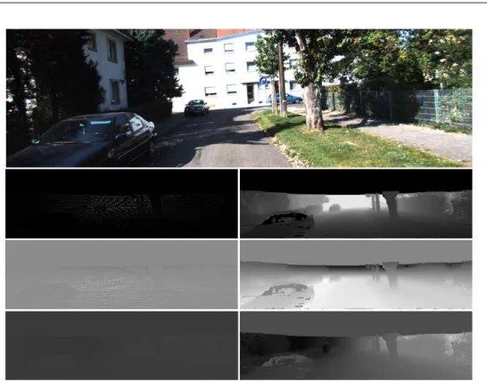
cloud, while discarding points such that λ < 0 or when [u, v] falls outside the image. This procedure generates three images, denoted as X, Y, and Z where each pixel contains the xc,yc, andzccoordinates of the 3D point that is projected into it. Given that the laser scanner has a limited number of channels, many pixels in the image are not associated with a valid detection, that is, there are no 3D points projected into them. In those cases, the pixel values are simply set to zero. The sparse LIDAR images are lastly upsampled using the procedure introduced by Premebidaet al. in [22] in order to obtain a dense input which is more suitable for fusion with the corresponding RGB images. Fig. 3.4 illustrates some examples of sparse and dense LIDAR images obtained using the above procedure.
Chapter
4
Applications
4.1
Road detection
A road detector is a system that estimates the free road surface that is avail-able for the future motion of the vehicle. Most state-of-the-art approaches carry out road detection using camera images and employ some kind of deep neural network (DNN) [13, 20, 18]. However, in order to achieve higher levels of driving automation, it will probably be necessary to use additional sensors besides cameras. One reason for this is that cameras are passive sensors and therefore cannot be relied upon in poor lighting conditions or at nighttime. Laser scanners (or LIDARs) on the other hand carry out sensing by emitting laser light pulses and timing their reflections. With this sensing mechanism, they can measure distances with high accuracy in any lighting condition. As shown in Fig. 4.1, the same scene captured by an RGB camera at different times during a day might show significant variability. On the other hand, those same scenes would appear rather similar to a laser scan-ner. With these considerations in mind, Paper I approached the problem of road detection using exclusively LIDAR point clouds, whereas Paper III investigated how to fuse RGB images and LIDAR data.
Road detection is commonly framed as a binary semantic segmentation task (see Sect. 2.3). The system is fed an image (e.g., RGB, point cloud top-view, etc.) and produces as output a confidence map that assigns to each pixel its probability of belonging to the road. Given the confidence map and the ground truth, several measures can then be computed for evaluating the system’s performance [7]. This work considers three in particular, namely
22 Chapter 4. Applications
Figure 4.1: Images of a scene captured at various times during the day [16]. As can be seen, there is significant appearance variability which makes the task of road detection using only RGB images particularly challenging or even impossible in certain conditions.
precision (PRE), recall (REC), and maximum F1-score (MaxF). These measures are computed as follows:
PRE = TP TP + FP, (4.1) REC = TP TP + FN, (4.2) MaxF = max τ 2× PRE(τ)×REC(τ) PRE(τ) + REC(τ), (4.3) where, TP denotes the true positives (road pixels correctly classified as road), FN represents the false negatives (road pixels classified as not-road), and FP denotes the false positives (not-road pixels classified as road). Lastly,
τ represents the classification threshold: Pixels in the confidence map with probability smaller than τ are assigned to the class not-road, whereas pixel with probability larger thanτ are classified as road.
4.1. Road detection 23
Convolution 3x3, stride 1, zero-padding + ELU
Dilated convolution 3x3, stride 1, zero-padding + spatial dropout + ELU
Max pooling 2x2, stride 2 Max unpooling Softmax
Convolution 1x1 W 200 H 400 D 32
Input Encoder Decoder Output
W 200 H 400 D 32 W 100 H 200 D 128 W 100 H 200 D 128 W 100 H 200 D 32 W 200 H 400 D 32 W 200 H 400 D 32 W 200 H 400 D 2 W 200 H 400 D 2 W 100 H 200 D 128 W 100 H 200 D 128 W 100 H 200 D 128 W 100 H 200 D 128 W 100 H 200 D 128 W 100 H 200 D 32 Context module
Conv 3x3, stride 1, zero-padding
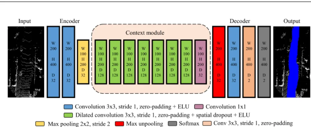
Figure 4.2: FCN architecture used in Paper I for road segmentation in point cloud top-views. The input consists of 6 stacked images encoding height and re-flectivity information (see Sect. 3.1). The output is a road confidence map. W represents the width, H denotes the height, and D is the number of feature maps.
4.1.1
LIDAR-only segmentation
Paper I considered only LIDAR point clouds, which were then transformed into top-view images using the procedure described in Sect. 3.1. A top-view perspective was chosen because both path planning and vehicle control are performed in this 2D world. Algorithms competing in the KITTI road bench-mark are also evaluated in this perspective [8]. Additionally, classification is simplified in comparison with the camera perspective where, for example, objects farther away appear smaller; in that case, an FCN would have to learn to recognize patterns at multiple scales thus requiring more training data and larger capacity. Fig. 4.2 shows the FCN architecture that was used for road segmentation. As can be seen, the general architecture resembles the encoder-decoder network that was described in Sect. 2.2.3. In this case, however, the encoder and decoder are shallower and include only one max pooling and one max unpooling layer, respectively. By keeping the feature maps at high resolution, it is possible to achieve higher segmentation accu-racy. The FCN also includes several dilated convolutional layers which are collectively denoted as acontext module. Dilated convolutions are sim-ilar to standard convolutions with the difference that one has to specify a parameter called dilation factor that determines how many units to skip when carrying out the convolution operation. By progressively increasing the dilation factor, it is possible to grow the receptive field of the network with fewer layers than would be required using standard convolutions.
24 Chapter 4. Applications
Convolution 3x3, stride 1, zero-padding 1+ ELU
W/2 H/2 D I N P U T W/2 H/2 D W/4 H/4 2*D W/4 H/4 2*D W/8 H/8 4*D W/2 H/2 D W/2 H/2 D W/4 H/4 2*D W/4 H/4 2*D W H 8 W H 3 S O F T M A X O U T P U T ENCODER DECODER CONTEXT MODULE
Convolution 4x4, stride 2, zero-padding 1+ ELU Convolution 3x3, stride 1,zero-padding 1 Deconvolution 4x4, stride 2, zero-padding 1+ ELU
L1 L2 L3 L4 L5 L15 L16 L17 L18 L19 L20 L21 L6 to L14
Figure 4.3: Base FCN architecture used in Paper III. The network consists of 20 layers and it is entirely convolutional. Both downsampling and upsampling are implemented using convolutional layers instead of max pooling and max unpooling layers as was the case in Paper I and II. Details about the context module can be found in Paper III.
RGB LIDAR LIDAR RGB L1 to L21 RGB LIDAR L1 to L20 L1 to L20 L20 LIDAR L20 RGB Conv OUT L21 OUT Lj-1 Lj-1 + *aj-1 *bj-1 + Lj Lj L20 L20 *a20 *b20 + L21 OUT
Early fusion Late fusion
Cross fusion RGB LIDAR Lcam Llid + *a1 *b1 + L2 L2 1 1
cam cam cam cam
lid lid lid lid
Figure 4.4: Fusion strategies investigated in Paper III for carrying our LIDAR-camera data fusion. In early fusion, the input tensors are concatenated and then processed together. In late fusion, two parallel branches each process one input tensor. Fusion happens deeper in the network at the decision level, just before the output layer. Cross fusion is also carried out by two parallel branches, however, in this case, trainable connections allow data integration at multiple depth levels.
4.1. Road detection 25
4.1.2
LIDAR-camera segmentation
Paper III also considered the road segmentation task using FCNs. In this case, however, LIDAR and camera data were fused together to achieve higher accuracy and robustness, in particular when dealing with challenging lighting conditions. To establish a direct correspondence between camera and LIDAR data, in this paper the point clouds were projected onto the camera plane and then upsampled using the procedure presented in Sect. 3.3. The base FCN architecture is shown in Fig. 4.3. As can be noticed, downsampling was performed by using 4×4 convolutions with stride 2 instead of max pooling layers. Given that the input images had a larger size compared to those used in Paper I, the encoder included three downsampling layers. Similarly, the decoder contained three upsampling layers.
Two common approaches for fusing multimodal data with CNNs are early fusion and late fusion. As shown in Fig. 4.4, early fusion simply involves concatenating the input tensors of each modality to create a multi-modal input tensor. In the specific case of LIDAR-camera fusion considered here, the input tensors are the RGB camera image and the ZYX dense image which, once stacked, become a tensor with 6 channels denoted as RGBZYX. This tensor is then processed with a single branch FCN.
Late fusion instead is carried out with a two-branch FCN (see Fig. 4.4), where each branch processes only one of the two input tensors. The actual fusion happens right before the output layer by feeding the processed single modality tensors to one last convolutional layer after concatenating them.
A contribution of Paper III was the introduction of a novel fusion strategy named cross fusionwhich is illustrated in the bottom panel of Fig. 4.4. As can be seen, the cross fusion network also consists of a two-branch FCN. In this case, however, the two branches are connected by trainable cross connections, denoted as aj and bj, j ∈ {1, . . . , N}, where N is the number
of layers. The underlying idea behind this strategy is to allow the FCN to learn to integrate multimodal information at any level of abstraction.
KITTI road benchmark results
The road detector developed in Papers I and III were evaluated on the KITTI road benchmark [8] to assess their performance against state-of-the-art algo-rithms. The results are reported in Table 4.1. LoDNN stands forLIDAR-only deep neural network and it is the system developed in Paper I. This approach
26 Chapter 4. Applications Table 4.1: KITTI road benchmark results (in %) on the urban road category. LidCamNet is the cross fusion FCN developed in Paper III. LoDNN is the LIDAR-only FCN introduced in Paper I. Only results of published methods are reported.
Rank Method MaxF PRE REC Time (s)
1 DFFA [15] 96.35 96.02 96.69 0.4 2 LidCamNet 96.03 96.23 95.83 0.15 3 RBNet [4] 94.97 94.94 95.01 0.18 4 StixelNet II [9] 94.88 92.97 96.87 1.2 6 LoDNN 94.07 92.81 95.37 0.018 14 LidarHisto [3] 90.67 93.06 88.41 0.1
obtained a MaxF score of 94.07% and outperformed by 3.4 percentage points the second best LIDAR-only system, LidarHisto. Furthemore, it is currently the algorithm with fastest inference. The cross fusion FCN introduced in Pa-per III is called LidCamNet which stands forLIDAR-Camera fusion network. This approach is currently the second best algorithm on the benchmark.
LidCamNet performed significantly better than LoDNN, the system de-veloped in Paper I. There might be several factors behind this gap: First and foremost, LidCamNet also used camera images, which in good lighting conditions provide rich discriminative clues for road detection. Another fac-tor that favored LidCamNet was that, in Paper III, the LIDAR images were upsampled, whereas the top-view images used in Paper I were sparse. One of the arguments put forward in Paper I was that road detection is more complex in the camera perspective because an FCN has to learn multiple scales. Given that in Paper III a LIDAR-only FCN (called ZYX-FCN) was also included in the experiments, it was possible to make some preliminary comparisons between LIDAR-based road detectors working in different per-spectives. ZYX-FCN could not be evaluated on the KITTI road benchmark (multiple submissions are discouraged) so a direct comparison of ZYX-FCN and LoDNN on the test set was not possible. However, the two FCNs were compared on the validation set used in Paper III: LoDNN achieved a MaxF score of 94.62% whereas ZYX-FCN obtained a score of 94.96%. The gap be-tween the two systems is not very large but it is noteworthy that ZYX-FCN performed better. In light of these results, it is clear that further experi-ments are warranted to determine whether a top-view perspective is indeed advantageous for carrying out road detection.
4.1. Road detection 27 94. 96 % 96.00% 95. 41 % 96.06 % 96.25% 95.21% 91. 81 % 95. 44 % 95.24% 96. 02 % 90.00% 91.00% 92.00% 93.00% 94.00% 95.00% 96.00% 97.00% 98.00% 99.00% 100.00%
ZYX RGB Early fusion Late fusion Cross fusion
MaxF [%] - validation MaxF [%] - challenging
Figure 4.5: Comparison of MaxF scores on the validation set and the challenging set.
Challenging driving scenes
An additional contribution of Paper III was to extend the KITTI road data set with additional scenes that were visually challenging. The purpose was to highlight the benefits of fusing LIDAR and camera data for achieving high accuracy in a wider spectrum of external conditions. The fusion FCNs previously described and two single modality FCNs were evaluated on a val-idation set selected from the KITTI road data set (fair weather and good lighting conditions) and on the challenging set mentioned above. The results of this experiment are reported in Fig. 4.5. As can be seen, the RGB-FCN performance was rather good on the validation set (96.00% MaxF) but, as expected, it decreased significantly on the challenging set (91.81% MaxF). All the FCNs that had access to LIDAR data achieved scores above 95% on the challenging set, thus confirming the usefulness of this sensor for robust road detection. The cross fusion FCN was again the most successful fusion strategy achieving a MaxF score above 96% in both the validation set and the challenging set.
28 Chapter 4. Applications
4.2
Driving path generation
The previous section dealt with the problem of road detection using camera and LIDAR sensors. Road detection, however, is just one among many tasks that must be carried out within the perception component of autonomous vehicles. The final goal is to detect and recognize all the driving factors in the vehicle’s surroundings so that a world model can be generated and then used for carrying out higher level functions such as path planning, decision making, and control.
An alternative paradigm, known as behavior reflex, instead proposes to learn all the driving functions with one single system. A famous example of this approach is ALVINN [21] developed by Pomerlau in 1989; in that work, a fully connected feedforward neural network with one hidden layer was trained to map low-resolution camera and range images to desired heading angles. An advantage of this type of approach is that the training data, which usually consists of sequences of camera images together with the corresponding ac-tions carried out by the driver (e.g., steering angle and acceleration), can be obtained automatically without the need of time-consuming hand-labeling. On the negative side, given that the system carries out all the driving func-tions, from perception to control, it is much more difficult to gain insight into its decision-making process and to predict how it will behave when presented with novel situations.
Paper II described an alternative approach where an FCN was trained to predict human-like driving paths for the future motion of a vehicle. Training examples were obtained automatically by processing the data logged during real driving sequences (e.g., LIDAR point clouds, GPS positions, etc.). In this way, a large data set was obtained without much effort. Also in this case, LIDAR top-view images were used as input for the FCN (see Sect. 3.1), however a larger region of interest was considered which covered the range [−30,30] meters in both the x and y directions. Additional input channels encoding information about the vehicle’s past motion and driving directions were generated by using the procedure described in Sect. 3.2. The FCN’s architecture was similar to the one used in Paper I, one of the main differences being that there were two max pooling layers instead of one in order to reduce the computational requirements because of the larger size of the input images. Several FCNs were trained using different combinations of input chan-nels for evaluating the benefits provided by individual sensor or information modalities. The FCN that only used LIDAR data obtained a score of 83.44%.
4.2. Driving path generation 29 Adding IMU provided a gain of 1.7 percentage points, whereas considering driving directions resulted in a gain of 2.3 percentage points. The FCN that used all the available data, that is, LIDAR point clouds, IMU information, and driving directions, obtained the best MaxF score of 88.13%. These re-sults showed that each modality contributed to improve performance and that the adopted data representation was appropriate for integrating multi-modal information.
Chapter
5
Conclusion and future work
5.1
Conclusion
This thesis has explored several applications of deep learning methods in the context of driving automation. It has been shown that CNNs, which are commonly used for processing camera images, can also be used effectively for working exclusively with LIDAR data (Paper I) or in combination with other sensors or information modalities (Papers II and III). The emphasis on the LIDAR sensor was motivated by its capacity to provide highly accurate range measurements in any lighting conditions; this alternative view of the environment can then be leveraged for making driving automation possible in a broader spectrum of external conditions.
It has been shown that sparse bird’s-eye view images can directly be used as input to an FCN for carrying out road segmentation (Paper I) with high ac-curacy and fast detection. The LIDAR-only deep neural network (LoDNN), achieved state-of-the-art performance with a MaxF score of 94.07% on the KITTI road benchmark, outperforming by a wide margin the second best LIDAR-based system.
By working in the same top-view perspective, a novel end-to-end learning system has been developed for generating driving paths (Paper II). Whereas a behavior reflex approach simply predicts the next driving action, a driving path specifies the vehicle’s future positions over a longer look-ahead horizon (30 meters, in this work). This makes the output of the proposed approach more interpretable and informative for further planning and decision-making. Additionally, the ground truth annotations for training the FCN are obtained
32 Chapter 5. Conclusion and future work in an automatic fashion thus allowing the generation of large training sets with no additional human effort and the possibility of continuous learning, that is, training the system while it is running in order for it to adapt to entirely novel situations. In order to exploit the visual pattern recognition capability of CNNs, information about the vehicle’s past motion and future destination were transformed into a spatial representation that allowed a direct integration with the point cloud top-views (Paper II).
Multimodal sensor fusion has also been investigated for the task of road detection. It has been shown that by combining camera images and LIDAR data, an FCN can carry out road segmentation in a wider range of external conditions than possible using only RGB images (Paper III). Besides evalu-ating two established fusion FCNs, early and late fusion, a novel multimodal FCN has been developed that can learn at what abstaction level and to what extent LIDAR and camera information should be fused. This approach was evaluated on the KITTI road benchmark for which it achieved state-of-the-art performance. In fact, it outperformed by almost two percentage points the system introduced in Paper I, a result that highlights the importance of developing multimodal approaches in the quest towards full driving automa-tion.
5.2
Future work
The approaches described in this thesis were all memory-less, that is, they processed each input independently of the previous ones. The integration of time in the system, either in the form of aggregated inputs (e.g., combining multiple LIDAR scans within one image) or by using networks with an in-ternal memory (such as recurrent neural networks) would likely improve the overall performance and robustness for all the considered tasks. For exam-ple, in its current formulation, the driving path generation FCN described in Paper II cannot know which objects are stationary and which ones are not, something that limits its applicability mostly to traffic-free scenarios.
Another important issue is the annotation of data. Supervised learning approaches, such as the ones presented here, need annotated training exam-ples which in general are very expensive to obtain in terms of time, money, and human effort. In Paper II, the problem of creating annotations was solved by using the GPS to recover the vehicle’s future driving path. A rele-vant topic for future work would be to devise similar strategies for automatic
5.2. Future work 33 or semi-automatic data labeling.
As was shown in Papers II and III, fusing multiple sensors and informa-tion modalities is generally beneficial for achieving better performance and robustness. In future work, it will be of high interest to investigate how addi-tional sensors (such as radars, stereo cameras, etc.) and information sources (e.g., high-definition maps) can be integrated within the proposed systems. A related topic will be the development of additional data representations that are suitable for multimodal data fusion.
Chapter
6
Summary of included papers
6.1
Paper I
This work was concerned with road detection using a LIDAR as the main sensor. The problem was cast as a semantic segmentation task and it was approached using a fully convolutional neural network (FCN). The FCN was designed to have a large receptive field and used high-resolution feature maps in order to achieve higher accuracy. Top-view images encoding several basic statistics were generated to summarize the information content of unstruc-tured point clouds into a format that was suitable for processing with the FCN. The proposed system carried out real-time inference at about 55 Hz us-ing a modern GPU and achieved state-of-the-art performance on the KITTI road benchmark reaching a MaxF score of 94.07% and outperforming by over 3.4 percentage points the second best LIDAR-only system.
6.2
Paper II
In this paper, a deep learning approach was developed to carry out driving path generation in LIDAR top-view images. This was accomplished by fus-ing LIDAR point clouds with GPS-IMU information and drivfus-ing directions using an FCN. The system was trained using as ground truth driving paths followed by human drivers. An advantage of this approach was that the an-notations were obtained automatically and therefore a large data set for su-pervised learning could be collected with limited effort. Several combinations
36 Chapter 6. Summary of included papers of inputs were considered to determine the effect of individual information modalities. The main result was that the FCN trained with all the available information (i.e., LIDAR, GPS-IMU, and driving directions) achieved the highest accuracy thus confirming that the chosen architecture and data rep-resentation were suitable for carrying out information fusion and that each modality contributed to the overall system performance.
6.3
Paper III
As Paper I, this work was also concerned with the task of road detection. However, in this case, the problem was solved by integrating RGB images and LIDAR point clouds that were projected onto the image plane. One of the main contributions of this work was the introduction of a novel fusion FCN architecture, called cross fusion, that allowed multimodal information fusion at any depth level in the network by using trainable cross connections. The cross fusion FCN outperformed two other established fusion approaches, early fusion and late fusion, as well as the single modality (RGB or LIDAR) FCNs. The system was evaluated on the KITTI road benchmark and ranked second with a MaxF score of 96.03%.
Bibliography
[1] V. Badrinarayanan, A. Handa, and R. Cipolla, Segnet: A deep convolutional encoder-decoder architecture for robust semantic pixel-wise labelling, arXiv preprint arXiv:1505.07293, (2015).
[2] M. Blanco, J. Atwood, S. Russell, T. Trimble, J. McClaf-ferty, and M. Perez, Automated vehicle crash rate comparison us-ing naturalistic data, tech. rep., Virginia Tech Transportation Institute, 2016.
[3] L. Chen, J. Yang, and H. Kong, Lidar-histogram for fast road and obstacle detection, in 2017 IEEE International Conference on Robotics and Automation (ICRA), May 2017, pp. 1343–1348.
[4] Z. Chen and Z. Chen, Rbnet: A deep neural network for unified road and road boundary detection, in International Conference on Neural Information Processing, Springer, 2017, pp. 677–687.
[5] D.-A. Clevert, T. Unterthiner, and S. Hochreiter, Fast and accurate deep network learning by exponential linear units (elus), CoRR, abs/1511.07289 (2015).
[6] S. Dahdah and K. McMahon,The true cost of road crashes: valuing life and the cost of a serious injury, International Road Assessment Programme, World Bank Global Road Safety Facility, (2008).
[7] T. Fawcett,An introduction to roc analysis, Pattern Recognition Let-ters, 27 (2006), pp. 861 – 874. ROC Analysis in Pattern Recognition.
38 BIBLIOGRAPHY [8] J. Fritsch, T. Kuhnl, and A. Geiger,A new performance measure and evaluation benchmark for road detection algorithms, in Intelligent Transportation Systems-(ITSC), 2013 16th International IEEE Confer-ence on, IEEE, 2013, pp. 1693–1700.
[9] N. Garnett, S. Silberstein, S. Oron, E. Fetaya, U. Verner, A. Ayash, V. Goldner, R. Cohen, K. Horn, and D. Levi, Real-time category-based and general obstacle detection for autonomous driv-ing, in Proceedings of the IEEE Conference on Computer Vision and Pattern Recognition, 2017, pp. 198–205.
[10] A. Geiger, P. Lenz, C. Stiller, and R. Urtasun, Vision meets robotics: The kitti dataset, The International Journal of Robotics Re-search, 32 (2013), pp. 1231–1237.
[11] I. Goodfellow, Y. Bengio, and A. Courville, Deep Learning, MIT Press, 2016.
[12] D. H. Hubel and T. N. Wiesel, Receptive fields, binocular interac-tion and funcinterac-tional architecture in the cat’s visual cortex, The Journal of physiology, 160 (1962), pp. 106–154.
[13] A. Laddha, M. K. Kocamaz, L. E. Navarro-Serment, and M. Hebert,Map-supervised road detection, in Intelligent Vehicles Sym-posium (IV), 2016 IEEE, IEEE, 2016, pp. 118–123.
[14] Y. LeCun, Y. Bengio, and G. Hinton,Deep learning, Nature, 521 (2015), pp. 436–444.
[15] X. Liu, Z. Deng, and G. Yang, Drivable road detection based on dilated fpn with feature aggregation, in 29th International Conference on Tools with Artificial Intelligence (ICTAI), IEEE, 2017.
[16] W. Maddern, G. Pascoe, C. Linegar, and P. Newman, 1 Year, 1000km: The Oxford RobotCar Dataset, The International Journal of Robotics Research (IJRR), 36 (2017), pp. 3–15.
[17] W. S. McCulloch and W. Pitts, A logical calculus of the ideas immanent in nervous activity, The bulletin of mathematical biophysics, 5 (1943), pp. 115–133.
BIBLIOGRAPHY 39 [18] R. Mohan, Deep deconvolutional networks for scene parsing, arXiv
preprint arXiv:1411.4101, (2014).
[19] V. Nair and G. E. Hinton, Rectified linear units improve restricted boltzmann machines, in Proceedings of the 27th International Confer-ence on Machine Learning (ICML), 2010, pp. 807–814.
[20] G. L. Oliveira, W. Burgard, and T. Brox,Efficient deep models for monocular road segmentation, in 2016 IEEE/RSJ International Con-ference on Intelligent Robots and Systems (IROS), Oct 2016, pp. 4885– 4891.
[21] D. A. Pomerleau, Alvinn: An autonomous land vehicle in a neural network, in Advances in Neural Information Processing Systems 1, D. S. Touretzky, ed., Morgan-Kaufmann, 1989, pp. 305–313.
[22] C. Premebida, J. Carreira, J. Batista, and U. Nunes, Pedes-trian detection combining rgb and dense lidar data, in 2014 IEEE/RSJ International Conference on Intelligent Robots and Systems, Sept 2014, pp. 4112–4117.
[23] F. Rosenblatt,The perceptron, a perceiving and recognizing automa-ton, Technical Report 85-460-1, (1957).
[24] D. E. Rumelhart, G. E. Hinton, and R. J. Williams, Learning representations by back-propagating errors, Nature, 323 (1986), pp. 533– 538.
[25] SAE On-Road Automated Vehicle Standards Committee and others, Taxonomy and definitions for terms related to on-road motor vehicle automated driving systems, SAE Standard J3016, (2014), pp. 01– 16.
[26] J. R. Treat, N. Tumbas, S. McDonald, D. Shinar, R. D. Hume, R. Mayer, R. Stansifer, and N. Castellan,Tri-level study of the causes of traffic accidents: final report, (1979).
[27] World Health Organization, Global status report on road safety 2015, World Health Organization, 2015.
![Figure 3.1: Top view of the sensor platform used for data collection of the KITTI Vision Benchmark Suite [10]](https://thumb-us.123doks.com/thumbv2/123dok_us/10191933.2921954/26.918.201.783.164.456/figure-sensor-platform-collection-kitti-vision-benchmark-suite.webp)

![Figure 4.1: Images of a scene captured at various times during the day [16].](https://thumb-us.123doks.com/thumbv2/123dok_us/10191933.2921954/34.918.200.785.187.480/figure-images-scene-captured-various-times-day.webp)