1
Improving accuracy of downscaling rainfall by combining predictions of
different statistical downscale models
Abstract
A flexible framework of multi-model of three statistical downscaling approaches was established in which predictions from these models were used as inputs to Artificial Neural Network (ANN). Traditional ANN, Simple Average Method (SAM), combining models (SDSM, Multiple linear regressions (MLR), Generalized Linear Model (GLM)) were applied to a studied site in North-western England. Model performance criteria of each of the primary and combining models were evaluated. The obtained results indicate that different downscaling methods can gain diverse usefulness and weakness in simulating various rainfall characteristics under different circumstances. The combining ANN model showed more adaptability by acquiring better overall performance, while GLM, MLR and showed comparable results and the SDSM reveals relatively less accurate results in modelling most of the rainfall amount. Furthermore traditional ANN has been tested and showed poor performance in reproducing the observed rainfall compared with above methods. The results also show that the superiority of the combining approach model over the single models is promising to be implemented to improve downscaling rainfall at a single site.
Keywords: Downscaling; SDSM; GLM; MLR; combining model; neural networks.
1. Introduction
One of the major findings of forecasting or prediction research over the last quarter century has been that greater predictive accuracy can often be achieved by combining forecasts or predictions from different methods or sources. The combining approach generally advocates the synchronous use of the forecast or prediction from a number of forecasting or predicting models to produce an overall combined or integrated forecast or prediction which can be used as an alternative to that produced by a single model. The basic hypothesis made in the combining approach is that different models capture different aspects of the data and hence the combination of these aspects would produce better variable estimates than those produced by any one of the individual models involved in the combination. Combination can be a process as straightforward as taking a simple average of the different forecasts, in which case the constituent forecasts are all weighted equally. Other, more sophisticated techniques are
2
available too, such as trying to estimate the optimal weights that should be attached to the individual forecasts, so that those that are likely to be the most accurate receive a greater weight in the averaging process. Within this context the current study has come by proposing the use of downscaled rainfall predicted by different downscaling models and combining them using simple average and artificial neural network methods.
Use of combining approach in different fields of forecasting is well documented and goes back to the 17th Century. Laplace (1818) has stated, when combining results of two forecasts, that “In combining the results of these two methods, one can obtain a result whose probability law of error will be more rapidly decreasing”. Since then different methods have been developed to find ‘optimal’ combinations of forecasts. Both simulation and empirical studies have been carried out to test the models and Bayesian interpretations have also been presented. The results have been virtually unanimous: combining multiple forecasts leads to increased forecast accuracy. This has been the result whether the forecasts are judgmental or statistical, econometric or extrapolation. Clement (1989); Hibon and Evgeniou (2005) have produced an excellent review for the methods used in combining forecasts and more information can be found in the named references and would not be repeated here. However, the methods used in the field of hydrology will be briefly discussed here.
Combining forecasts of different rainfall-runoff models was first used by Shamseldin (1997) and Shamseldin et al. (1997). This has then been followed by several studies which have dealt with multi-model combination of hydrological models (e.g. Xiong et al., 2001; Abrahart and See, 2002; Coulibaly et al., 2005; Ajami et al., 2006; Viney et al., 2009). As the nature of the combination function is unknown and no theory exists to analytically derive the combination function from a hydrological or physical point of view, the previous studies have used empirical data-driven modelling to derive the combination function and such use is very appropriate. In all the aforementioned studies both linear and non-linear combination functions have been used (e.g. linear regression, neural network and fuzzy logic) to produce multi-model river flows. Application results from these studies have demonstrated the potential capabilities of the multi-model combination approach in improving the accuracy and reliability of hydrological modelling results and have laid the foundation for further use of this approach in rainfall-runoff modelling (Shamseldin, 1997; See and Openshaw, 2000; Xiong et al., 2001; Coulibaly et al., 2005). The success stories of using the combining
3
approach in the field of rainfall-runoff forecasting have formed great motivations for the current study.
Rainfall is one of the most difficult elements of the hydrological cycle to forecast (French et al., 1992) and great uncertainties still affect the performances of both stochastic and deterministic rainfall prediction models. Interesting perspectives for the future rainfall are offered by numerical global circulation models (GCMs), however, up until now, they unfortunately do not seem able to provide accurate rainfall forecasts at the temporal and spatial resolution required by many hydrologic applications (Brath, 1999). To overcome the problem of spatial and temporal data limitations, rainfall disaggregation and simulation approach (particularly for climate change studies) for the coarse resolution of the GCMs is generally used. This approach is generally referred to as downscaling.
During the last two decades, extensive research has been conducted on downscaling methods and their applications. Numerous techniques and methods have been proposed and used which can be broadly divided into statistical and dynamical methods. Statistical downscaling is the most widely used method in downscaling climate variables from GCMs. It relates large- scale climate variables (predictors) to regional and local variables (predictands). The large-scale outputs of the GCM simulation are then fed into this statistical model to estimate the corresponding local and regional climate characteristics (Wilby et al., 2004). (In list stated 200
Different techniques for statistical downscaling (SD) have been employed including regression- based techniques, weather pattern classification and weather generators. The fundamental assumption used in the SD techniques is that the derived relationships between the observed predictors (climate variables) and predictand (i.e. rainfall) will remain constant under conditions of climate change and that the relationships are time-invariant (Yarnal et al., 2001; Fowler et al., 2007). One of the primary advantages of SD techniques is that they are computationally inexpensive and thus can be easily applied to outputs from different GCM experiments (Wilby et al., 2004).
Several regression-based techniques have been used to downscale the precipitation with different capabilities for each method including linear and non-linear regression. Beuchat et al. (2012); Fealy and Sweeney (2007) used Generalized Linear Models (GLMs) which perform well in reproducing historical rainfall statistics in Switzerland and Ireland,
4
respectively. Muluye (2012) employed the hybrid (SDSM), ANN, and nearest neighbor-based approaches (KNN) in Canada with greater skills for ANN models. Another study carried by Hassan and Harun (2012) shows that the SDSM model can be well acceptable in regards to its performance in downscaling of the daily and annual rainfall in Malaysia. Results from three downscaling methods (multiple linear regressions, multiple non-linear regression, and stochastic weather generator) were successfully used by Hashmi et al. (2012) in climate impact study and the outcome is encouraging any future attempts for combining the results of multiple statistical downscaling methods. Moreover many other studies used linear regression (Busuioc et al., 2008; Goubanova et al., 2010), nonparametric regression based on splines, generalized additive models (Vrac et al., 2007; Salameh et al., 2009) in downscaling rainfall for climate change impact and adaptations studies and obtained good results.
In the present study, the multi-model combining approach has been applied to the area of downscaling rainfall from the outputs of GCM. The main objective is to improve downscaling rainfall prediction by combining predictions from different statistical downscaling models. The models used to downscale rainfall in the studied site are the Multiple Linear Regression (MLR), the Generalised Linear Model (GLM), the SDSM (Wilby et al., 2002). The combining models used are the Simple Average Method (SAM) and the Artificial Neural Network (ANN) which both compared with traditional ANN (no combination approach).
2. Study Area and Data
The Crewe drainage area in North West of England (NW), Figure 1, is selected for this study. The exposure of the NW region to westerly maritime air masses and the presence of extensive areas of high ground mean that the region is considered as one of the wettest places in the UK, with average annual rainfall over 3200mm. The rainfall in the Crewe area is recorded at Worelston Station (WR).
Two principal data sets were employed during the calibration and validation of the daily rainfall downscale models. Firstly, the observed daily rainfall data set, collected from WR station was obtained from the Environment Agency for England & Wales, for the period 1961–1990. Secondly, the large-scale observed climatic predictors data set was obtained from the National Centre for Environment Predictions (NCEP/NCAR). Originally at resolution of
5
2.50x2.50 degrees, this data was re-gridded to confirm with output of the HadCM3 GCM that has grid resolution of 2.50x3.750.Thus Inverse Distance Weighted (IDW) method (Willmott et al.1985) of interpolation was applied prior to the use of GCM output in prediction. IDW interpolation explicitly implements the assumption that things that are close to one another are more alike than those that are farther apart. To predict a value for any unmeasured location, IDW will use the measured values surrounding the prediction location. Those measured values closest to the prediction location will have more influence on the predicted value than those farther away. Thus, IDW assumes that each measured point has a local influence that diminishes with distance. It weights the points closer to the prediction location greater than those farther away, hence the name inverse distance weighted.
The two sets of data were needed to build the rainfall downscale model of the drainage area.The relationships between large scale atmospheric data and local variables are important for simulating future rainfall conditioned by climate projections. There are 26 large scale climate variables used in this study which were assessed for their influence on rainfall at the WR station for winter, spring, summer and autumn seasons. These variables were used for the purpose of constructing the rainfall model (observed). Observed daily predictor variables have been normalised with respect to their 1961-1990 means and standard deviations.
3. Methodology
The methodology followed in this study consists of three steps. The first step was screening for predictors of rainfall in the studied site using NCEP large scale climatic variables. The second step involved building of three seasonal rainfall models using the SDSDM, MLR and GLM downscale models with the data in period 1961–1975 used for calibration and that in period 1976–1990 used for validation. The third step involved combining of the predictions obtained from the three downscale models using Simple Average Method (SAM) and Artificial Neural Network combining method (ANN). Below is a brief description for each of these steps and the models used.
3.1 Screening for Predictors
Selection of appropriate predictors is the most important step in rainfall downscaling exercise. It would generally not be useful to include all potential predictors in a final model. This is because the predictor variables are almost always mutually correlated, so that the full set of potential predictors contains redundant information (Wilks, 1995).
6
The predictors - rainfall relations in this research are formed based on correlation coefficients between them. Stepwise regression is applied in the present study for selection of predictors from the NCEP climatic data as it has been shown as a powerful method by many previous studies (e.g. Huth, 1999; Harpham and Wilby, 2005). The pool of predictors used were daily values of 26 variables comprising surface pressure, temperature and humidity as well as upper air measures of wind speed and direction, vorticity, divergence, humidity, temperature and geo-potential height.
The screening process has yielded the most powerful and parsimonious seasonal model possible consisting of 8 predictors presented in Table 1. In order to remove any inconsistencies associated with the presence of small rainfall values, a threshold of 0.3mm was applied to the data as rainfall values less than this threshold are considered to be dry days and represented with zero. Those equal to or greater than the threshold were considered wet days.
3.2 Downscale Models
3.2.1 SDSM
SDSM uses a hybrid stochastic weather generator and multi-linear regression method to simulate local precipitation at each station conditional on regional circulation and atmospheric moisture predictors (Harpham and Wilby, 2005). Thus, it has the ability to capture the inter-annual variability better than other statistical downscaling approaches, e.g. weather generators, weather typing (Wilby et al., 2002). SDSM is a combination of a stochastic weather generator approach and a transfer function model (Wilby et al., 2002) needing two types of daily data. The first type corresponds to local predictands of interest (e.g. temperature, precipitation, etc.) and the second type corresponds to the data of large scale predictors (NCEP and GCM) of a grid box closest to the study area. Correlation and partial correlation analysis is performed in SDSM between the predictand of interest and predictors to select a set of predictors most relevant for the site in question (Wilby et al., 2002). Although SDSM has its own function for predictors screening, however this function was not used in the present study.
SDSM models rainfall in two steps, the first step is developing of an occurrence rainfall model using the screened predictors as described in equation 1 (Wilby et al., 1999):
7 O𝑖 = 𝛼0+ ∑ 𝛼𝑗𝑝𝑗𝑖
𝑛
𝑗=1 (1) The second step is rainfall amount model which uses the same screened predictors in a regression model as described in equation 2 (Wilby et al., 1999):
𝑅𝑆𝐷𝑆𝑀𝑖 = 𝛽
0+ ∑ 𝛽𝑗𝑝𝑗𝑖 𝑛
𝑗=1 + 𝑒𝑖 (2) where, Oi is the conditional probability of daily rainfall occurrence on dayi, RiSDSMare daily
rainfall amounts, pij are predictors, n is number of predictors, α and β are model parameters
estimated by dual simplex algorithm and ei is modelling error.
The version of SDSM used in this study is version 5.1.1 which is freely downloaded from the software website. A full description of the software, its various functions and mathematical formulation can be found in the User Manual (Wilby and Dawson, 2013).
3.2.2 MLR
Multiple Linear Regression (MLR) is one of the most widely used forms of regression. In the present study the rainfall is modelled in MLR as amount only (no occurrence process) by solving a linear model of the form:
𝑅𝑀𝐿𝑅𝑖 = 𝛽
0+ ∑ 𝛽𝑗𝑝𝑗𝑖 𝑛
𝑗=1 + 𝜀𝑖 (3) where, εi ~ N(0, σ2) is a Gaussian error term with variance σ2, all other symbols in equation 3
have the same meaning as in equations 1 and 2.
The MLR model developed in this study was programmed in MATLAB and used method of maximum likelihood to estimate model parameters. The main problem with MLR model is that it tries to model the conditional mean, which is not best suited for predicting extremes. However, the focus in this study is prediction of rainfall time series not only the extremes and hence use of MLR is justified.
3.2.3 GLM
Generalised Linear Model (GLM) belongs to linear regression family, but differs from the MLR by assuming a distribution other than the normal distribution for the response variable
Riin equation 3 above. The GLM form used in the present study relates the response variable
(Ri), whose distribution has a vector mean μ = (μ1, . . .,μm) to one or more covariates (p) via the relationships (Fealy and Sweeney 2007):
8 𝜇 = 𝐸(𝑅) (4) 𝑔(𝜇) = 𝜈 (5) 𝑅𝐺𝐿𝑀𝑖 = 𝜈 = 𝛽 0+ ∑ 𝛽𝑗𝑝𝑗𝑖 𝑛 𝑗=1 (6) A log link function, ɡ(μ), and gamma distribution were employed for the purposes of modelling the rainfall and β are model parameters. While the mixed exponential distribution has been found to provide a better fit to rainfall amounts (Wilks and Wilby, 1999) the relationship between the mean and variance for this distribution makes it difficult to incorporate into a GLM. Nonetheless, the gamma distribution GLM has been found to be a good fit to precipitation amounts in a number of regions (Chandler and Wheater, 2002) and hence used here.
The GLM model developed in this study was programmed in MATLAB and used method of maximum likelihood to estimate model parameters.
3.3 Combining models
3.3.1 SAM
The Simple Average Method (SAM) takes the arithmetic average of the forecast or prediction obtained from the three downscale models, treating the forecasts or prediction of each model of having the same weight in the combined forecast. This can be expressed as follows:
𝑅𝑆𝐴𝑀𝑖 = 1
3{𝑅𝑆𝐷𝑆𝑀
𝑖 + 𝑅
𝑀𝐿𝑅𝑖 + 𝑅𝐺𝐿𝑀𝑖 } (6) The SAM is a naïve forecast combination method, which can work very well when the constituent models have practically the same level of performance; it is more sensible to use it purely as a baseline against which the results of more sophisticated combination methods can be compared.
3.3.2 ANN
The Artificial Neural Network method uses the forecast or prediction obtained from the three downscale models as inputs to a Multi-Layer feed Forward Artificial Neural Network (MLF-ANN) model. The structure of the MLF-ANN model used in this study consists of an input layer, an output layer and two “hidden” layers located between the input and the output
9
layers as shown in Figure 2. Each neuron of a particular layer has connection pathways to all the neurons in the following adjacent layer, but none to those of its own layer or to those of the previous layer (if any). Likewise, nodes in non-adjacent layers are unconnected. In the output layer, there is only one neuron, for the single output. The number of neurons in the input and output layers is determined by the number of elements in the external input array and output array of the network, respectively. The number of neurons in the hidden layers is determined by trial and error (Hammerstorm, 1993) for the best performing model as presented in Table 2. The final output, RANN, from the network shown in Figure 2 is obtained
by the following equation:
𝑅𝐴𝑁𝑁 = 𝑓𝑜𝑢𝑡(∑ 𝜃𝑛𝑘 𝑘𝑓ℎ𝑖𝑑𝑑𝑒𝑛2{∑ 𝛽𝑚𝑗 𝑗𝑘𝑓ℎ𝑖𝑑𝑑𝑒𝑛1(∑ 𝑅𝑖3 𝑖𝛼𝑖𝑗 + 𝛼0𝑗) + 𝛽0𝑗} + 𝜃0) (7) Where,
Ri The input to the network from the primary downscale models.
αij The connection weights between nodes of the input and hidden layer.
βjk The connection weights between nodes of hidden layer 1 and hidden layer 2.
θk The connection weights between nodes of hidden layer 2 and outer layer.
α0j β0j and θ0 are neuron thresholds (or baseflow) in hidden 1, hidden 2 and output layers,
respectively.
m and n are numbers of neurons in hidden layer 1 and hidden layer 2.
fhidden1, fhidden2 and fout are the logistic, logistic and identity transfers functions for hidden layer
1, hidden layer 2 and output layer, respectively.
The weights and threshold values constitute the parameters of the network, which are usually estimated by calibrating (or training) of the network. This is usually achieved by minimizing the sum of the squares of the differences between the network output series (RANN), and the
corresponding observed rainfall, Robs, using nonlinear optimization algorithms. In the present
research, the faster back-propagation algorithm of Levenberg-Marquardt (Yadav et al., 2010) of MATLAB 7.11 was used, which was designed to speed up the training process.
Moreover, traditional ANN with same predictors inputs as in the three models SDSM, MLR and GLM has been applied and trained with same training algorithm of CANN. This will investigate its own capabilities compared with the other methods and the combining approaches.
10
4. Results and Discussion
The methodology described above was sequentially followed. Observed daily rainfall time series obtained for Worleston (WR) station for 30 years was used together with the large-scale observed climatic variables of NCEP data; correspond to the North Wales Grid (NW) of HadCM GCM, to establish seasonal predictant –predictors relationship in the studied site. Using the method of stepwise regression, the appropriate predictors for daily rainfall in this station are presented in Table 1. The predictors were found to be the same for all four seasons.
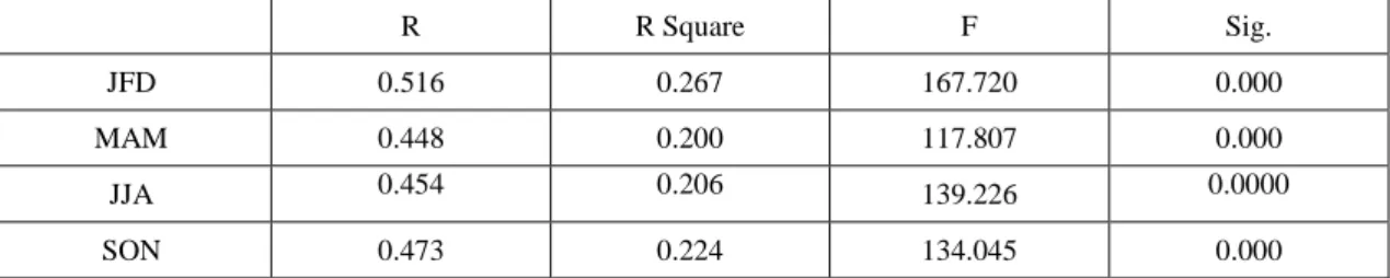
Stepwise linear regression is a method of regressing multiple variables while simultaneously removing those that aren't important which has been done through SPSS. Stepwise regression essentially does multiple regression a number of times, each time removing the weakest correlated variable. At the end the variables that explain the distribution best will be left. Results in Table 1a show R (correlation), R2 (coefficient of determination), F-value and significance level of that F-value. The F-value is statistically significant with typically p
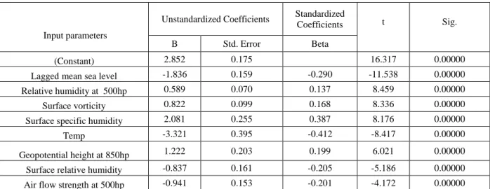
< .05, this signifies that the models did a good job of predicting the outcome variable and that there is a significant relationship between the set of predictors and the dependent variable (rainfall).
After the evaluation of the F-value and R2, it is important to evaluate the regression beta coefficients: unstandardized and standardized. The beta coefficients can be negative or positive, have a t-value and significance of that t-value associated with it. If the beta coefficient is not statistically significant (i.e., the t-value is not significant), no statistical significance can be interpreted from that predictor. If the regression beta coefficient is positive, the interpretation is that for every 1-unit increase in the predictor variable, the dependent variable will increase by the unstandardized beta coefficient value. Results for the model coefficients and their significant have been presented in Table 2b-e which show Sig. figures below 0.05. Then the selected predictors were then used to build primary rainfall downscale models using each of the modelling methods described in Section 3.2.
The observed daily rainfall data set (1961-1990) with corresponding selected predictors have been divided into two sets comprising calibration (period 1961-1975) and verification (period 1976-1990) sets. All of the primary models were calibrated and verified using the same calibration and validation periods. Having built the three SDSM, MLR and GLM primary downscale models for each season, the combining SAM and CANN seasonal models were
11
built using outputs from these primary models as inputs. The SAM model was built as simple arithmetic average of the three primary downscale models, whereas the ANN model was developed using the network structure shown in Figure 2. Two types of activation functions have been used, the log-sigmoid for the hidden layer and linear transfer function in the output layer. Appropriate numbers of neurons in each of the two hidden layers of the network are presented in Table 2a for each seasonal model. The two hidden layers have been used after many trials because one layer failed to give best fit for the data and hence it leads to a lesser accurate model. Moreover, same preditors that used in the three statistical downscale models were directly applied to ANN which results in network structures in Table 2b (traditional ANN). Performance estimates such as cross-validation by splitting the data into calibration and validation dataset has been used in both traditional ANN and CANN models with 90% of the data were selected randomly for calibration and 10% for validation in Matlab.
Capabilities of CANN and traditional one in terms of generalization and avoiding overfitting have been also investigated by comparing the number of models parameters (connections weights and biases) with number of data points set that used to train the network. Table 2 a-b showed that the ANNs used less parameters than the data used which increase the confidence of using the ANNs for simulation and prediction. Furthermore the early stopping approach has been used to prevent overfitting and improve the generalization during the training so the run automatically will stop the training if ANN experience any overfitting.
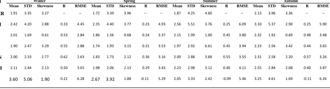
The efficiency and ability of each primary and combining model to predict rainfall amount that best match the observed rainfall are expressed here in terms of correlation coefficient (R) and root mean square error (RMSE) and presented in Table 3. Table 3 shows that, without exception, the ANN combining model (CANN) produces daily rainfall estimates that possess a higher correlation coefficient (R) with the observed rainfall and a lower RMSE than the correlation coefficient values associated with the primary models and even the SAM combining model (CSAM). The SAM combining approach is relatively unskilful compared to the CANN approach and even to the other three methods while traditional ANN showed least skilful compared to all. Among the primary downscale models, the GLM and MLR primary models perform better than the SDSM in estimating daily rainfall at the station.
In addition to the statistics and efficiency results presented in Table 3, five more diagnostic tests are performed on the three primary, two combining downscale models and traditional
12
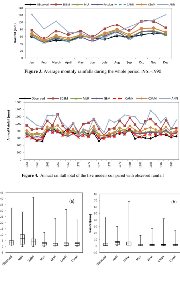
ANN to ensure their suitability for downscaling future rainfall in the study site. These are demonstrated in figures 3, 4, 5, 6 and 7 for calibration and validation data set. Figure 3 shows comparison plots of the average monthly rainfall amount between the observed and rainfall simulated by the five models for the whole period 1961 – 1990. The plots demonstrate a good degree of agreement between the observed and simulated average monthly rainfalls by the combining ANN model. It can clearly be deduced from these plots that the combining ANN model is able to reproduce the monthly rainfall and therefore it is an improvement over the other primary downscale models.
Figure 4 shows the inter-annual variability for rainfall in the studied site, between the observed and simulated series for the whole period 1961-1990. The total yearly values would appear to have been adequately captured by the combining ANN model better than the other three primary models, the combining SAM model and traditional ANN. Therefore these results, together with those in figure 3, demonstrate that the combining ANN (CANN) model is more reliable in reproducing the observed rainfall which is an important requirement when assessing climate impacts on hydrological systems.
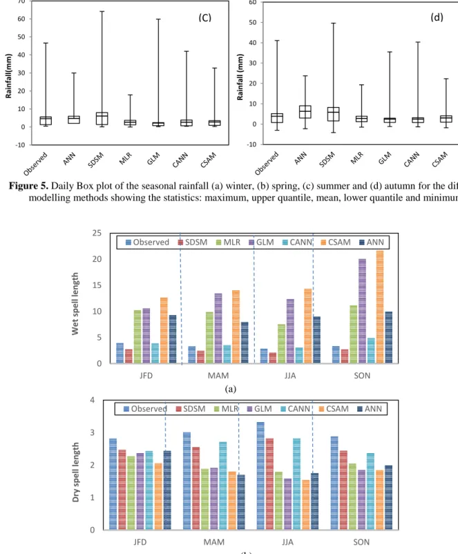
In figure 5 the Daily Box plots of the simulated seasonal rainfall characteristics is represented as small vertical bars showing some statistics of rainfal series simulated by different downscale models. The plotted statistics are measures of how much spread there is around the average; with closeness of the simulated statistic value to the corresponding observed statisitc value indicates good representation for the observed spread of the data. By viewing the daily box plots of the seasonal rainfall in figure 5, the error bars correspond to the CANN model appear much closer to the observed ones for all seasons. Those correspond to the MLR model rank the lowest. This is a clear indication that the combining CANN model produces rainfall much similar to the observed one in terms of data spreading around the mean. It is an additional evidence that combining predictions from different dowscale models can produce better results.
Figures 6a and 6b show annual average dry and wet spells, resepctively, yielded by different downscale models in comparison to the observed one. A thresold of 0.3 mm is used to distinguish a dry day from a wet one. In figure 6a the average seasonal dry spells computed from the rainfall simulated by the SDSM, MLR, GLM, CSAM and traditional ANN models are lower than the observed ones, whereas the average seasonal dry spells computed from the
13
combining ANN model is much closer to the obserserved one. Conversly, in figure 6b, the average wet spell computed from the raifall simulated by the MLR, GLM, traditional ANN and CSAM models are significantly overestimated the observed ones, whereas the SDSM and the combining ANN produced an average seasonal wet days reasonably matching the observed ones. The closeness of the average seasonal dry and wet spells produced by the combining ANN model to the observed ones, is another desireable property needed in downscaling model results when used in climate impact modelling.
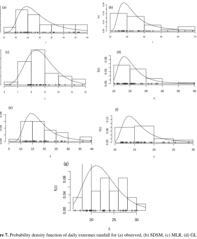
The last diagonistic test for examing the performance of the different primary models and the combining ones is the the probability desnsity functions, pdf, for the simulated annual maximum rainfall serie (AM) obtained from each model. Figures 7a, 7b, 7c, 7d, 7e and 7f, show shapes of the pdf produced the AM series by each model. Concerning the shape of the distribution, it can be observed that the pdf of the observed rainfall skews slightly to the left while those from the SDSM and GLM skew to the left more than the observed one while CSAM skew to left with less degree compared to observed one. The pdf of the MLR and traditional ANN model tends to resemble the normal distribution, whereas that of the combining ANN skews slightly to the left similar to the pdf of observed rainfall. Similarly, the boundaries of the extremes (along the x-axis) are different for different downscale models, with those of the observed and the combining ANN are much closer to each other. The analogy in skewness of the pdf shape and closeness in the extremes boundaries between the observed and the combining ANN suggest that the variability of rainfall produced by the combining ANN is much similar to those of the observed ones. .
5. Conclusions
Three statistical downscaling primary models have been compared with two combining models in terms of their ability to downscale daily rainfall over a selected site in Northwest England. Daily observed rainfall data for the period 1961 – 1990, together with the observed NCEP data, was used to calibrate and verify the models. A number of diagnostic tests or parameters was used to measure the ability and performance of each primary and combining model to downscale the daily rainfall. The statistical results showed the combining ANN models performed better in downscaling seasonal rainfall much closer to the observed series than the primary SDSM, GLM and MLR models, traditional ANN and the combining SAM model. The other diagnostic tests of monthly average rainfall, the inter-annual variability, the daily box plots, the annual average dry/wet spells and the probability density function plots,
14
which are important requirements for assessing climate change impact, have all revealed that the combining ANN model generally performs better in reproducing the inter-annual variability and magnitude of the rainfall in comparison to the other primary and combining models. While SDSM show much closer performance to CANN in term of reproducing wet and dry spell length however it is significantly overestimate the annual variability, average monthly, and daily statistics of the rainfall. This means that SDSM can be able to simulate the occurrence properly but not the amount unlike CANN which is good for both.
Overall, this paper highlights the importance of acknowledging limitations and advantages of different statistical downscaling methods, and also implies that there is a room for improvements by combining these models. The results obtained for this studied catchment are promising as well as encouraging and can be extended to multiple site and regions in the future.
Acknowledgment
The authors would like to acknowledge the help received from the Environment Agency for England and Wales and the Met Office UK in form of data received and discussion taken place during the period of this study.
References
Abrahart, R. J., See, L. M., 2002. Multi-model data fusion for river flow forecasting: an evaluation of six alternative methods based on two contrasting catchments. Hydrology andEarth System Sciences. 6(4), 655-670.
Ajami, N. K., Duan, Q., Gao, X., Sorooshian, S., 2006. Multimodel combination techniques for analysis of hydrological simulations: application to Distributed Model Intercomparison Project results. Journal of
Hydrometeorology. 7, 755–768.
Beuchat, X., Schaefli, B., Soutter, M., Mermoud, A., 2012. A robust framework for probabilistic precipitations downscaling from an ensemble of climate predictions applied to Switzerland, J. Geophys. Res. 117, D03115.
Brath, A., 1999. On the role of numerical weather prediction models in real-time flood forecasting. Proceedings of the International Workshop on River Basin Modeling: Management and Flood Mitigation, September 25–26, Monselice, Italy, pp. 249–259.
Busuioc, A., Tomozeiu, R., Cacciamani, C., 2008. Statistical downscaling model based on canonical correlation analysis for winter extreme precipitation events in the Emilia-Romania region, Int. J. Climatol.28, 449–464.
15
Chandler, R.E., Wheater, H.S., 2002. Analysis of rainfall variability using generalized linear models: A case study from the west of Ireland. Water Resources Research. 38, 1192, doi:10.1029/2001WR000906.
Clement, R. L., 1989. Combining forecasts: A review and annotated bibliography. International Journal of Forecasting. 5, 559-583.
Coulibaly, P., Hache, M., Fortin, V., Bobee, B., 2005. Improving Daily reservoir inflow forecasts with model combination. ASCE Journal of Hydrologic Engineering. 10(2), 91-99.
Fealy, R., Sweeney, J., 2007. Statistical downscaling of precipitation for Selection of sites in Ireland employing a generalised linear modelling approach. International Journal of Climatology. 27, 2083-2094.
Fowler, H.J., Blenkinsop, S., Tebaldi, C., 2007. Linking climate change modelling to impacts studies: recent advances in downscaling techniques for hydrological modelling. International Journal of climatology.
27:1547-1578.
French, M.N., Krajewski, W.F., Cuykendall, R.R., 1992. Rainfall forecasting in space and time using a neural network. J. Hydrol. 137, 1–31.
Goubanova, K., Echevin, V., Dewitte, B., Codron, F., Takahashi, K., Terray, P., Vrac, M., 2010. Statistical downscaling of sea-surface wind over the Peru-Chile upwelling region: Diagnosing the impact of climate change from the IPSL-CM4 model, Clim. Dyn.36(7–8), 1365–1378.
Hammerstorm, D., 1993. Working with Neural Networks. IEEE Spectrum 46-53.
Harpham, C., Wilby, RL., 2005. Multi-site downscaling of heavy daily precipitation occurrence and amounts.
Journal of Hydrology 312: 235–255.
Hashmi, M.Z., Shamseldin, Y.A., Melville, B.W., 2012. Statistically downscaled probabilistic multi-model ensemble projections of precipitation change in a watershed. Hydrological process Journal, DOI:10.1002/hyp.8413.
Hassan, Z., Harun, S., 2012. Application of Statistical Downscaling Model for Long Lead Rainfall Prediction in Kurau River Catchment of Malaysia. Malaysian Journal of Civil Engineering. 24(1), 1-12.
Hibon, Michele., Evgeniou, Theodoros., 2005. To combine or not to combine: selecting among forecasts and their combinations. International Journal of Forecasting. 21, 15-24.
Huth, R., 1999. Statistical downscaling in central Europe: evaluation of methods and potential predictors. Clim. Res. J. 13, 91–101.
16
Muluye., G.Y., 2012. Comparison of statistical methods for downscaling daily precipitation. Journal of Hydroinformatics. doi:10.2166/hydro.2012.197.
Salameh, T., Drobinski, P., Vrac, M., Naveau, P., 2009. Statistical downscaling of near surface wind field over complex terrain in southern France, Meteorol. Atmos. Phys.103, 253–265.
See, L., Openshaw, S., 2000. A hybrid multi-model approach to river level forecasting. Hydrological Sciences
Journal, 45(4), 523-536.
Shamseldin, A. Y., O'Connor, K. M., and Liang, G. C., 1997. Methods for combining the outputs of different rainfall-runofff models. Journal of Hydrology, 197, 203-229.
Shamseldin, A. Y., 1997. Application of a neural network technique to rainfall-runoff modelling, J. Hydrol., 199, 272-294.
Viney, N. R., Bormann, H., Breuer, L., Bronstert, A., Croke, B. F. W., Frede, H. G., T., Hubrechts, L., Huisman, J. A., Jakeman, A. J., Kite, G. A., Lanini, J., Leavesley, G., Lettenmaier, D. P., Lindstrom, G., Seibert, J., Sivapalan, M., and Willems, P., 2009. Assessing the impact of land use change on hydrology by ensemble modeling (LUCHEM) II: Ensemble combinations and predictions. Advances in Water Resources, 32, 147-158.
Vrac, M., P. Naveau., 2007. Stochastic downscaling of precipitation: From dry events to heavy rainfalls, Water
Resour. Res., 43, W07402, doi: 10.1029/2006WR005308.
Wilby, R.L., Hay, L.E., Leavesley, G.H., 1999. A comparison of downscaled and raw GCM output: implications for climate change scenarios in the San Juan River basin, Colorado. Journal of Hydrology 225, 67e91.
Wilks, D.S., and R.L. Wilby., 1999. The weather generation game: a review of stochastic weather models.Progress in Physical Geography, 23, 329-357.
Wilby., RL., Dawso, C.W., Barrow. E.M., 2002. SDSM – A decision support tool for the assessment of regional climate change impacts. Environmental Modelling and Software 17:147–159.
Wilby, R.L., Charles, S.P., Zorita, E., Timbal, B., Whetton, P., Mearns, L.O., 2004. Guideline for use of climate scenarios development from statistical downscaling methods. Environmental agency, King College London, CSIRO land and water, GKSS, Bureau of Meteorology. CSIRO atmospheric research and National centre for atmospheric research.
Wilby, R. L., Dawson, C. W., 2013. Statistical Downscaling Model (SDSM), User Manual. Version 5.1.1
17
Willmott, C. J., C. M. Rowe, and Y. Mintz, 1985. Climatology of the Terrestrial Seasonal Water Cycle. Journal of Climatology, 5, 589-606.
Xiong, L., Shamseldin, A. Y., O'Connor, K. M., 2001. A non-linear combination of the forecasts of rainfall-runoff models by the first-order Takagi-Sugeno fuzzy system. Journal of Hydrology. 245(1-4), 196-217.
Yadav, D., Naresh, R., Sharma ,V., 2010. Stream flow forecasting using Levenberg-Marquardt algorithm approach. IJWREE. 3(1), 30-40.
Yarnal, B., Comrie, A., Frakes, B., Brown, D., 2001. Developments and prospects in synoptic climatology. International Journal of Climatology. 21, 1923–1950.
18
Table 1a: Stepwise regression models performance summary for the four seasons
R R Square F Sig.
JFD 0.516 0.267 167.720 0.000
MAM 0.448 0.200 117.807 0.000
JJA 0.454 0.206 139.226 0.0000
SON 0.473 0.224 134.045 0.000
Table 1b: Stepwise regression coefficients and significance for each predictor in Winter at 5% significance level
Input parameters
Unstandardized Coefficients Standardized
Coefficients t Sig. B Std. Error Beta
(Constant) 1.694 0.195 8.670 0.00000 Lagged mean sea level -1.074 0.074 -0.406 -14.545 0.00000 Surface specific humidity 2.443 0.491 0.466 4.976 0.00000 Air flow strength at 500hp 0.503 0.048 0.167 10.464 0.00000 Surface vorticity 0.689 0.061 0.225 11.370 0.00000 Geopotential height at 850hp 0.753 0.090 0.268 8.381 0.00000 Relative humidity at 500hp 0.330 0.052 0.109 6.300 0.00000 Temp -2.406 0.526 -0.391 -4.571 0.00001 Surface relative humidity -0.345 0.115 -0.065 -2.998 0.00273
Table 1c: Stepwise regression coefficients and significance for each predictor in Spring at 5% significance
Input parameters Unstandardized Coefficients Standardized Coefficients t Sig. B Std. Error Beta (Constant) 2.100 0.073 28.599 0.00000 ncepmslpeu+1 -0.920 0.095 -0.259 -9.719 0.00000 ncepr500eu 0.563 0.057 0.169 9.875 0.00000 ncepp__zeu 0.683 0.071 0.199 9.663 0.00000 ncepp850eu 0.620 0.119 0.171 5.232 0.00000 ncepp5_feu 0.173 0.054 0.048 3.184 0.00147 ncepshumeu 1.919 0.286 0.368 6.716 0.00000 nceptempeu -1.720 0.283 -0.342 -6.077 0.00000 nceprhumeu -0.575 0.124 -0.165 -4.640 0.00000
19
Table 1d: Stepwise regression coefficients and significance for each predictor in Summer at 5% significance level Input parameters Unstandardized Coefficients Standardized Coefficients t Sig. B Std. Error Beta (Constant) 2.852 0.175 16.317 0.00000 Lagged mean sea level -1.836 0.159 -0.290 -11.538 0.00000 Relative humidity at 500hp 0.589 0.070 0.137 8.459 0.00000 Surface vorticity 0.822 0.099 0.168 8.336 0.00000 Surface specific humidity 2.081 0.255 0.387 8.176 0.00000 Temp -3.321 0.395 -0.412 -8.417 0.00000
Geopotential height at 850hp 1.222 0.203 0.199 6.021 0.00000 Surface relative humidity -0.837 0.161 -0.205 -5.186 0.00000 Air flow strength at 500hp -0.941 0.153 -0.201 -4.172 0.00000
Table 1e: Stepwise regression coefficients and significance for each predictor in Autumn at 5% significance level Input parameters Unstandardized Coefficients Standardized Coefficients t Sig. B Std. Error Beta (Constant) 1.996 0.072 27.681 0.00000 Lagged mean sea level -1.219 0.105 -0.306 -11.554 0.00000 Relative humidity at 500hp 0.537 0.066 0.136 8.099 0.00000 Surface vorticity 0.770 0.083 0.195 9.232 0.00000 Air flow strength at 500hp 0.479 0.061 0.122 7.845 0.00000 Geopotential height at 850hp 0.665 0.134 0.163 4.971 0.00000 Temp -2.030 0.352 -0.359 -5.761 0.00000 Surface specific humidity 1.517 0.299 0.326 5.067 0.00000
20
Table 2a: Structure ofcombining ANN model in terms of number of hidden neurons for 8 inputs and one out puts
Season
Hidden layer Neurons
Total No. of model parameters (connections/biases)
Total No. of data points in training set JFD 25, 25 901 1353 MAM 20, 15 511 1380 JJA 25, 25 901 1380 SON 20, 20 601 1365
Table 2b: Structure of traditonal ANN model in terms of number of hidden neurons for 8 inputs and one out puts
Season Hidden layer Neurons Total No. of model parameters
(connections/biases)
Total No. of data points in training set
JFD 7 71 1335
MAM 13 131 1380
JJA 16 161 1380
21
Table 3: Models Statistics and Efficiency for Calibration and Validation periods
Model Winter Spring Summer Autumn
Mean STD Skewness R RMSE Mean STD Skewness R RMSE Mean STD Skewness R RMSE Mean STD Skewness R RMSE
OBSER 1.91 3.35 3.27 ─ ─ 1.72 3.39 3.96 ─ ─ 1.87 4.25 4.60 ─ ─ 2.13 3.96 3.36 ─ ─ SDSM 2.42 4.20 2.88 0.33 4.45 2.35 4.40 3.77 0.23 4.93 2.56 5.51 3.76 0.25 6.09 3.10 5.37 2.90 0.25 5.90 MLR 2.01 1.69 0.61 0.53 2.84 1.86 1.56 0.68 0.24 3.37 2.15 1.99 1.00 0.45 3.80 2.32 1.92 0.69 0.48 3.48 GLM 1.90 2.47 3.29 0.55 2.88 1.74 1.93 3.15 0.21 3.53 1.97 2.92 6.61 0.45 3.94 2.23 2.56 3.42 0.44 3.65 CANN 2.00 2.33 2.77 0.62 2.63 1.83 1.73 2.12 0.36 3.16 2.00 2.88 3.68 0.55 3.55 2.31 2.58 2.20 0.57 3.26 CSAM 2.11 2.44 2.13 0.50 3.01 1.98 2.06 2.13 0.29 3.43 2.23 2.98 3.12 0.40 4.11 2.55 2.84 2.08 0.40 3.87 ANN 3.60 5.06 1.90 0.21 6.28 2.67 3.92 1.88 -0.11 5.29 2.05 3.33 2.42 -0.09 5.46 3.25 4.61 1.69 -0.11 6.26
22
Figure 1. Crewe study area in North West of England
Figure 2. Combined ANN structure Input layer RSDSM RMLR . . . . . . RGLM CANN Hidden layers Output layer
23
Figure 3. Average monthly rainfalls during the whole period 1961-1990
Figure 4. Annual rainfall total of the five models compared with observed rainfall 0 20 40 60 80 100 120 140
Jan Feb March April May Jun July Aug Sep Oct Nov Dec
R ai nfa ll (m m )
Observed SDSM MLR Possion CANN CSAM ANN
0 200 400 600 800 1000 1200 1400 1600 1 9 6 1 1 9 6 3 1 9 6 5 1 9 6 7 1 9 6 9 1 9 7 1 1 9 7 3 1 9 7 5 1 97 7 1 9 7 9 1 9 8 1 1 9 8 3 1 9 8 5 1 9 8 7 1 9 8 9 A nnual R ai nfa ll (m m )
Observed SDSM MLR GLM CANN CSAM ANN
-5 0 5 10 15 20 25 30 35 40 45 R ai nfa ll (m m ) (a) -10 0 10 20 30 40 50 60 70 80 R ai nfa ll(m m ) (b)
24
Figure 5. Daily Box plot of the seasonal rainfall (a) winter, (b) spring, (c) summer and (d) autumn for the different modelling methods showing the statistics: maximum, upper quantile, mean, lower quantile and minimum
(a)
(b)
Figure 6. Average wet (a) and dry (b) spell length for the four seasons during calibration and verification period 1961-1990 -10 0 10 20 30 40 50 60 70 R ai nfa ll(m m ) -10 0 10 20 30 40 50 60 R ai nfa ll (m m ) 0 5 10 15 20 25
JFD MAM JJA SON
We t spel l l e n gth
Observed SDSM MLR GLM CANN CSAM ANN
0 1 2 3 4
JFD MAM JJA SON
D ry spel l l e n gth
Observed SDSM MLR GLM CANN CSAM ANN
25
Figure 7. Probability density function of daily extremes rainfall for (a) observed, (b) SDSM, (c) MLR, (d) GLM, (e) Combining ANN(f) Combining SAM and (g) traditional ANN during calibration verification period 1961-1990
0.0 0.2 0.4 0.6 0.8 1.0 0 .0 0 .2 0 .4 0 .6 0 .8 Probability Plot Empirical M o d e l 20 30 40 50 20 25 30 35 40 45 Quantile Plot Model E m p ir ic a l 20 40 60 80 100 Return Period R e tu rn L e v e l 0.1 1 10 100 1000
Return Level Plot Density Plot
z f( z ) 15 20 25 30 35 40 45 50 0 .0 0 0 .0 2 0 .0 4 0 .0 6 0.0 0.2 0.4 0.6 0.8 1.0 0 .0 0 .2 0 .4 0 .6 0 .8 Probability Plot Empirical M o d e l 30 40 50 60 70 30 40 50 60 70 Quantile Plot Model E m p ir ic a l 50 100 150 200 250 Return Period R e tu rn L e v e l 0.1 1 10 100 1000
Return Level Plot Density Plot
z f( z ) 20 30 40 50 60 70 0 .0 0 0 .0 2 0 .0 4 0 .0 6 0.0 0.2 0.4 0.6 0.8 1.0 0 .0 0 .2 0 .4 0 .6 0 .8 1 .0 Probability Plot Empirical M o d e l 7 8 9 10 11 7 8 9 10 11 12 Quantile Plot Model E m p ir ic a l 7 8 9 10 12 Return Period R e tu rn L e v e l 0.1 1 10 100 1000
Return Level Plot Density Plot
z f( z ) 6 7 8 9 10 11 12 0 .0 0 .1 0 .2 0 .3 0 .4 0.0 0.2 0.4 0.6 0.8 1.0 0 .0 0 .4 0 .8 Probability Plot Empirical M o d e l 15 20 25 30 35 40 45 10 30 50 Quantile Plot Model E m p ir ic a l 20 40 60 80 Return Period R e tu rn L e v e l 0.1 1 10 100 1000
Return Level Plot Density Plot
z f( z ) 10 20 30 40 50 60 0 .0 0 0 .0 3 0 .0 6 0.0 0.2 0.4 0.6 0.8 1.0 0 .0 0 .4 0 .8 Probability Plot Empirical M o d e l 10 15 20 25 30 35 10 20 30 40 Quantile Plot Model E m p ir ic a l 20 40 60 80 Return Period R e tu rn L e v e l 0.1 1 10 100 1000
Return Level Plot Density Plot
z f( z ) 5 10 15 20 25 30 35 40 0 .0 0 0 .0 4 0 .0 8 0.0 0.2 0.4 0.6 0.8 1.0 0 .2 0 .6 1 .0 Probability Plot Empirical M o d e l 15 20 25 15 20 25 Quantile Plot Model E m p ir ic a l 10 30 50 Return Period R e tu rn L e v e l 0.1 1 10 100 1000
Return Level Plot Density Plot
z f( z ) 10 15 20 25 30 0 .0 0 0 .0 6 0 .1 2 0.0 0.2 0.4 0.6 0.8 1.0 0 .0 0 .2 0 .4 0 .6 0 .8 Probability Plot Empirical M o d e l 18 20 22 24 26 28 30 16 20 24 28 Quantile Plot Model E m p ir ic a l 15 20 25 30 35 40 Return Period R e tu rn L e v e l 0.1 1 10 100 1000
Return Level Plot Density Plot
z f( z ) 20 25 30 0 .0 0 0 .0 4 0 .0 8 (a) (b) (c) (d) (e) (f) (g)