IET Research Journals
Regular Paper
Partially coupled gradient estimation
algorithm for multivariable equation-error
autoregressive moving average systems
using the data filtering technique
ISSN 1751-8644 doi: 0000000000 www.ietdl.org
Qinyao Liu
1, Feng Ding
1,2,3,∗, Ling Xu
1, Erfu Yang
41Key Laboratory of Advanced Process Control for Light Industry (Ministry of Education), School of Internet of Things Engineering, Jiangnan University, Wuxi 214122, People’s Republic of China
2College of Automation and Electronic Engineering, Qingdao University of Science and Technology, Qingdao 266061, People’s Republic of China 3Department of Mathematics, King Abdulaziz University, Jeddah 21589, Saudi Arabia
4Department of Design, Manufacture and Engineering Management, Space Mechatronic Systems Technology Laboratory, Strathclyde Space Institute, University of Strathclyde, Glasgow G1 1XJ, Scotland, United Kingdom
* E-mail: [email protected]
Abstract:System identification provides many convenient and useful methods for engineering modeling. This paper targets the parameter identification problems for multivariable equation-error autoregressive moving average systems. To reduce the influence of the colored noises on the parameter estimation, the data filtering technique is adopted to filter the input and output data, and to transform the original system into a filtered system with white noises. Then we decompose the filtered system into several subsystems and develop a filtering based partially-coupled generalized extended stochastic gradient algorithm via the coupling concept. In contrast to the multivariable generalized extended stochastic gradient algorithm, the proposed algorithm can give more accurate parameter estimates. Finally, the effectiveness of the proposed algorithm is well demonstrated by simulation examples.
1 Introduction
Mathematical models can describe the dynamic behavior of a sys-tem as a function of time and exist in various fields, such as fault diagnosis [1, 2], telecommunication transmission [3–5], con-trol system [6, 7] and signal processing [8, 9]. In most cases, it is not easy to analyse the whole system and to construct the mathe-matical model based on the analytic approach. Therefore, system identification becomes the first choice when people model a system [10–12], and has a wide application in both linear [13] and nonlinear systems [14–17]. For the multiple-input and multiple-output Box-Jenkins model with disturbances, a two-stage identification method was developed by using the residual model of Kalman filter [18]. Separating the parameters to be estimated into a linear part and a nonlinear part is a common idea to solve the nonlinear least squares problems. Based on this method, Gan et al. eliminated the linear parameters through the orthogonal projection and presented a vari-able projection algorithm for the radial basis function network-based autoregressive with exogenous inputs model [19].
During the past decade, a great deal of attention has been given to multivariable system identification [20, 21] for the reason that many modern industrial processes are multivariable systems [22]. Applying the scalar system identification methods to multivariable systems may give poor performances, because multivariable systems have high-dimensional variables, complicated structures and many uncertain disturbances [23]. It attracts an increasing interest for researchers to explore more valid methods for multivariable systems [24, 25]. When dealing with the multivariable systems with colored noises, the data filtering technique can be applied to reduce the influ-ence of the noise and improve the estimation accuracy [26–28]. In [29], a filtering based multi-innovation extended stochastic gradi-ent algorithm was developed for improving the parameter estimation accuracy of the multivariable system with the moving average noise. To simplify the identification model for multivariable systems, the hierarchical identification principle provides a new idea to this prob-lem [30, 31]. The hierarchical identification, which is also known as
the decomposition identification, is to decompose a large-scale sys-tem into several small size subsyssys-tems with fewer variables. How-ever, after the decomposition of some multivariable systems, there are some parameter coupled relations between the subsystems. In this case, we link the parameter estimates inside the subsystems and identify each subsystem based on the coupling identification concept [32]. The coupling identification concept can avoid the redundant estimates and improve the computational efficiency for multivariable systems. In this literature, Ding et al. combined the coupling con-cept and the gradient search to estimate the non-uniformly sampled systems and obtained a highly computational efficiency algorithm [33]. For nonlinear multivariable output-error moving average sys-tems, a partially coupled extended stochastic gradient algorithm was presented by using the decomposition technique and the coupling concept [34]. In the previous work [35], we applied the hierar-chical identification principle to multivariable system and used the coupling concept to solve the redundant computation.
This work studies the recursive identification methods of multi-variable equation-error autoregressive moving average systems by using the data filtering technique and the coupling identification con-cept. In view of the colored noises, we first design a filter according to the model structure. By filtering the input-output data, the multi-variable system is divided into a noise model and a filtered system model. Next, the filtered system model is decomposed into sev-eral sub-models on the basis of the number of outputs. However, a major challenge encountered in estimating the parameters is that there are some unmeasurable variables inside the noise system and the sub-models. To obtain the feasible algorithm, we establish some auxiliary models and replace the unknown variables with the outputs of these models. Then, a filtering based partially-coupled general-ized extended stochastic gradient (F-PC-GESG) algorithm is derived by using the coupling concept and the auxiliary model. Compared with the multivariable generalized extended stochastic gradient (M-GESG) algorithm, the F-PC-GESG algorithm gives more accurate parameter estimates under the same noise level. In addition, we
introduce a forgetting factor to improve the performance of the F-PC-GESG algorithm.
The outline of this paper is as follows. The symbols and the iden-tification model for the multivariable equation-error autoregressive moving average system are given in Section 2. Section 3 derives the filtered identification models and presents the F-PC-GESG algorithm based on the data filtering technique and the coupling con-cept. Section 4 proposes the M-GESG algorithm and gives some comparisons with the F-PC-GESG algorithm. The numerical simula-tions are shown to verify the effectiveness of the proposed algorithms in Section 5. Section 6 offers some concluding remarks to end the paper.
2 Problem formulation
In this section, we state the identification problems and derive the hierarchical identification model for multivariable equation-error autoregressive moving average systems. Let us start by introducing some symbols used in this paper.“A=:X”or“X:=A”stands for
“Ais defined asX”; the superscript T stands for the vector/matrix transpose; the symbolImdenotes an identity matrix of appropri-ate size (m×m);1mstands for anm-dimensional column vector whose elements are 1;1m×n represents a matrix of sizem×n whose elements are 1; the symbol ⊗ represents the Kronecker product, for example,A:=aij∈Rm×n,B:=bij∈Rp×q,A⊗
B= [aijB]∈R(mp)×(nq), in general,A⊗B̸=B⊗A;col[X] is defined as a vector formed by all columns of matrix X and arranged in order, for example,X:= [x1,x2,· · ·,xn]∈Rm×n,
xi∈Rm(i= 1,2,· · ·, n),col[X] := [xT1,xT2,· · ·,xTn]T∈Rmn;
ˆ
θ(t)denotes the estimate ofθat timet; the norm of a matrix (or a column vector)Xis defined by∥X∥2:= tr[XXT].
Consider the following multivariable equation-error autoregres-sive moving average system which is also called the multi-variable controlled autoregressive autoregressive moving average (CARARMA) system:
A(z)y(t) =B(z)u(t) +D(z)
C(z)v(t), (1)
wherey(t) := [y1(t), y2(t),· · ·,ym(t)]T∈Rm refers to them -dimensional output vector, u(t) := [u1(t), u2(t), · · ·, ur(t)]T∈ Rr
denotes ther-dimensional input vector,v(t) := [v1(t), v2(t),
· · ·, vm(t)]T∈Rm is a white noise vector, A(z) and B(z) are matrix polynomials in the unit backward shift operator z−1
[z−1u(t) =u(t−1)],C(z) and D(z) are scalar polynomials in
z−1, and they are defined as
A(z) :=Im+A1z−1+A2z−2+· · ·+Anaz− na, B(z) :=B1z−1+B2z−2+· · ·+Bnbz− nb, C(z) := 1 +c1z−1+c2z−2+· · ·+cncz− nc, D(z) := 1 +d1z−1+d2z−2+· · ·+dndz− nd.
Define an intermediate variable
w(t) :=D(z)
C(z)v(t). (2)
Letn:=mna+rnb, define the parameter matrixθ, the parameter vectorρ, the information vectorφ(t)and the information matrix
ψ(t)as θT:= [A1,A2,· · ·,Ana,B1,B2,· · ·,Bnb]∈R m×n , ρ:= [c1, c2,· · ·, cnc, d1, d2,· · ·, dnd] T∈Rnc+nd, φ(t) := [−yT(t−1),−yT(t−2),· · ·,−yT(t−na), uT(t−1),uT(t−2),· · ·,uT(t−nb)]T∈Rn, ψ(t) := [−w(t−1),−w(t−2),· · ·,−w(t−nc), v(t−1),v(t−2),· · ·,v(t−nd)]∈Rm×(nc+nd).
Through the above definitions,w(t)can be expressed as different forms, w(t) = [1−C(z)]w(t) +D(z)v(t) =− nc ∑ i=1 ciw(t−i) + nd ∑ i=1 div(t−i) +v(t) =ψ(t)ρ+v(t). (3) According to (1) and (2),w(t)can also be described as
w(t) =A(z)y(t)−B(z)u(t)
=y(t)−θTφ(t). (4) Substituting (2)–(4) into (1), we can obtain the following hierarchi-cal identification model,
y(t) = [Im−A(z)]y(t) +B(z)u(t) +w(t)
=θTφ(t) +w(t)
=ψ(t)ρ+θTφ(t) +v(t). (5) Equation (5) has a parameter vectorρand a parameter matrixθ. In order to simplify the model in (5), combine the information vector
φ(t)with the information matrixψ(t)to construct an information matrixΦ(t)by means of the Kronecker product:
Φ(t) := [ψ(t),φT(t)⊗Im]∈Rm×n0, n0:=nc+nd+mn. Define a new parameter vector:
ϑ:= [ ρ col[θT] ] ∈Rn0.
Then Equation (5) can be rewritten as a pseudo-linear regressive model:
y(t) =Φ(t)ϑ+v(t). (6) Equation (6) is the identification model for the multivariable CARARMA system in (1).
Remark 1: For the identification model in (6), the parameter vector
ϑcontains all the parameters to be estimated. Although some algo-rithms can estimate the parameter vectorϑ, the high-dimensional parameter vector and information matrix result in a heavy compu-tational burden and poor performance of these algorithms. On the other hand, the information matrix Φ(t)consists of the unknown intermediate variablesw(t−j)and the noise termsv(t−j). The objective of this paper is to present a new effective algorithm using the observation datau(t)andy(t). By employing the coupling iden-tification concept and the data filtering technique, the new algorithm can deal with the unknown variables and give more accurate param-eter estimates for the multivariable CARARMA system in (1). Since this paper focuses on the parameter estimation, we assume that the orders and the initial values are known, that is to say, the ordersm,r,
na,nb,ncandndare known andy(t) =0,u(t) =0andv(t) =0 fort60.
3 The filtering based partially-coupled
generalized extended stochastic gradient algorithm It is worth noting that the system considered in this paper is disturbed by the autoregressive moving average noise (i.e., colored noise). In order to reduce the impact of the noise, we introduce the data fil-tering technique here to obtain more accurate estimates. The basic idea is to use a filter to filter the input-output data and to decompose the original identification model into two models which contain a filtered system model and a noise model. Then we further divide the system model into a series of subsystems according to the number of
outputs and identify each subsystem based on the coupled relations in part of the parameters between subsystems. From the above-mentioned idea, we deduce the filtering based partially-coupled generalized extended stochastic gradient (F-PC-GESG) algorithm in this section.
Define the filtered input vectoruf(t)and the filtered output vector
yf(t)as
uf(t) :=C(z)u(t)∈Rr, yf(t) :=C(z)y(t)∈Rm.
Multiplying both sides of (1) byC(z)gives
A(z)C(z)y(t) =B(z)C(z)u(t) +D(z)v(t),
or
A(z)yf(t) =B(z)uf(t) +D(z)v(t). (7)
Define the noise parameter vectord, the information matrixϕ(t)
and the filtered information vectorφf(t): d:= [d1, d2,· · ·, dnd]
T∈Rnd,
ϕ(t) := [v(t−1),v(t−2),· · ·,v(t−nd)]∈Rm×nd,
φf(t) := [−yfT(t−1),−yTf(t−2),· · ·,−yTf(t−na),
uTf(t−1),uTf(t−2),· · ·,uTf(t−nb)]T∈Rn. Then Equation (7) can be modified as
yf(t) = [Im−A(z)]yf(t) +B(z)uf(t) +D(z)v(t) =ϕ(t)d+θTφf(t) +v(t). (8) LetϕTi(t)∈R1×ndbe theith row of the information matrixϕ(t):
ϕ(t) := [ϕ1(t),ϕ2(t),· · ·,ϕm(t)]T∈Rm×nd. Similarly, letθi(t)∈Rnbe theith column of the parameter matrix
θandyfi(t)be theith element of the filtered output vectoryf(t),
that is
θ:= [θ1,θ2,· · ·,θm]∈Rn×m,
yf(t) := [yf1(t), yf2(t),· · ·, yfm(t)]T∈Rm. Equation (8) can be explicitly written as
yf1(t) yf2(t) .. . yfm(t) = ϕT1(t) ϕT2(t) .. . ϕTm(t) d+ θT1 θT2 .. . θTm φf(t) + v1(t) v2(t) .. . vm(t) . (9)
Then we can decompose the filtered system in (9) intomfiltered subsystem identification models
yfi(t) =ϕTi(t)d+θ T iφf(t) +vi(t) =ϕTi(t)d+φ T f(t)θi+vi(t) = [ϕTi(t),φTf(t)] [ d θi ] +vi(t), i= 1,2,· · ·, m. (10) Define the subsystem information vector
ψi(t) := [ ϕi(t) φf(t) ] ∈Rn+nd.
The filtered subsystems in (10) can be expressed as
yfi(t) =ψTi(t) [ d θi ] +vi(t). (11)
From the definition ofw(t), we can obtain
C(z)w(t) =D(z)v(t). (12) Rewrite Equation (12) as the following form
w(t) =Ω(t)c+ϕ(t)d+v(t),
where Ω(t) is the noise information matrix and c is the noise parameter vector:
Ω(t) := [−w(t−1),−w(t−2),· · ·,−w(t−nc)]∈Rm×nc,
c:= [c1, c2,· · ·, cnc]
T∈Rnc.
Define an intermediate variable wn(t) :=w(t)−ϕ(t)d∈Rm. Then another similar formula can be derived forwn(t):
wn(t) =Ω(t)c+v(t). (13) Equations (11) and (13) are the filter hierarchical subsystem identifi-cation model and the noise model for the multivariable CARARMA system in (1). Compared with the identification model in (6), the fil-ter identification models divide the system paramefil-ters into two parts, Equation (11) contains the parameter vectorsθiandd, and the noise vectorcis in the noise model (13). Note that the filtered subsystem identification model is disturbed by the white noisev(t), in other word, we transform the origin system in (1) which has colored noise tomfiltered subsystem models with white noise and a noise model. Based on the filtered subsystem identification model (11) and the noise model (13), using the negative gradient search principle gives
[ ˆ d(t) ˆ θi(t) ] = [ ˆ d(t−1) ˆ θi(t−1) ] +ψi(t) r1(t) × { yfi(t)−ψTi(t) [ ˆ d(t−1) ˆ θi(t−1) ]} , (14) r1,i(t) =r1,i(t−1) +∥ψi(t)∥ 2 , (15) ˆ c(t) = ˆc(t−1) +Ω T(t) r2(t) [wn(t)−Ω(t)ˆc(t−1)], (16) r2(t) =r2(t−1) +∥Ω(t)∥2. (17)
Note that the information vectorψi(t) (i= 1,2,· · ·, m)contains the unknown variable v(t−j), and the information matrix Ω(t)
is made of the unmeasured intermediate variablew(t−j). More-over, since the parameter vector cis unknown, we cannot obtain the filtered input vectoruf(t)and the filtered output vectoryf(t).
All these imply that the above relations are impossible to generate the estimatesdˆ(t),θˆi(t)andcˆ(t)directly. The solution here is to replace the unknown variablesw(t−j)andv(t−j)with the out-putswˆ(t−j)andvˆ(t−j)of the auxiliary models. Then we can obtain the estimates ofΩ(t)andϕ(t):
ˆ
Ω(t) := [−wˆ(t−1),−wˆ(t−2),· · ·,−wˆ(t−nc)]∈Rm×nc,
ˆ
ϕ(t) := [ˆv(t−1),vˆ(t−2),· · ·,vˆ(t−nd)]
= [ ˆϕ1(t),ϕˆ2(t),· · ·,ϕˆm(t)]T∈Rm×nd.
According to Equation (4), replacingθwith its estimateθˆ(t)gives
ˆ
w(t) =y(t)−θˆT(t)φ(t).
From the definition of the intermediate variable wn(t), replacing
w(t)anddwithwˆ(t−1)anddˆ(t−1)gives
ˆ
wn(t) = ˆw(t−1)−ϕˆ(t) ˆd(t−1)
Use the parameter estimate
ˆ
c(t) := [ˆc1(t),ˆc2(t),· · ·,ˆcnc(t)]
T∈Rnc×1
to construct the estimate ofC(z):
ˆ
C(t, z) = 1 + ˆc1(t)z−1+ ˆc2(t)z−2+· · ·+ ˆcnc(t)z−
nc.
Here, we use the filterCˆ(t, z)to filter the input vector and the output vector, and obtain the estimates of the filtered input vectoruf(t)and
the filtered output vectoryf(t): ˆ uf(t) = ˆC(t, z)u(t) =u(t) + ˆc1(t)u(t−1) +· · ·+ ˆcnc(t)u(t−nc) =u(t) + [u(t−1),u(t−2),· · ·,u(t−nc)]ˆc(t), ˆ yf(t) = ˆC(t, z)y(t) =y(t) + ˆc1(t)y(t−1) +· · ·+ ˆcnc(t)y(t−nc) =y(t) + [y(t−1),y(t−2),· · ·,y(t−nc)]ˆc(t) = [ˆyf1(t),yˆf2(t),· · ·,yˆfm(t)]T. Then the estimate ofφf(t)can be defined as
ˆ φf(t) := [−yˆ T f(t−1),−yˆ T f(t−2),· · ·,−yˆ T f(t−na), ˆ uTf(t−1),uˆ T f(t−2),· · ·,uˆ T f(t−nb)]T∈Rn. Subsequently, the information vectorψˆi(t)is constructed by using
ˆ ϕi(t)andφˆf(t): ˆ ψi(t) = [ ˆ ϕi(t) ˆ φf(t) ] ∈Rn+nd.
According to Equation (8), replacingyf(t),ϕ(t) and φf(t) with
their estimatesyfˆ(t),ϕˆ(t) andφˆf(t), we can get the estimate of v(t):
ˆ
v(t) = ˆyf(t)−ϕˆ(t) ˆd(t)−ˆθ
T
(t) ˆφf(t). (18) Besides the unknown variables involved in (14)–(17), there is still a problem that each subsystem will produce a parameter estimation vectordˆ(t)of the same parameter vectordat each timet. In order to make it clear, we usedˆi(t)to represent the estimate of Subsystem
i. Then, replaceyfi(t)andψi(t)in (14)–(15) with their estimates
ˆ
yfi(t) and ψˆi(t), and replace wn(t) andΩ(t) in (16)–(17) with their estimates wnˆ (t) and Ωˆ(t). Through these replacement, we modify Equations (14)–(17) as [ˆ di(t) ˆ θi(t) ] = [ˆ di(t−1) ˆ θi(t−1) ] + ˆ ψi(t) r1,i(t) × { ˆ yfi(t)−ψˆ T i(t) [ˆ di(t−1) ˆ θi(t−1) ]} , (19) r1,i(t) =r1,i(t−1) +∥ψˆi(t)∥ 2 , i= 1,2,· · ·, m, (20) ˆ c(t) = ˆc(t−1) +Ωˆ T (t) r2(t) [ ˆwn(t)−Ωˆ(t)ˆc(t−1)], (21) r2(t) =r2(t−1) +∥Ωˆ(t)∥2. (22)
It is worth noting that there are dˆ1(t), dˆ2(t), · · ·, dˆm(t) for
i= 1,2,· · ·, m in (19)–(22), and this leads to many redundant parameter estimates. However, cutting down the redundant param-eter estimates and improving the paramparam-eter estimation accuracy are our aims to explore new identification methods. In general, we usu-ally desire that the proposed algorithm is convergent, that is to say, the parameter estimates approach their true values as the timet
increases. Therefore, we can assume that the parameter estimate
ˆ
di−1(t) is closer to the true value than the parameter estimate ˆ
di(t−1). Based on the coupling identification concept, for i=
2,3,· · ·, m, usedˆi−1(t) to replacedˆi(t−1)and for i= 1, use
ˆ
dm(t−1)to replaced1ˆ(t−1). Thus, we can obtain the following F-PC-GESG algorithm: [ˆ di(t) ˆ θi(t) ] = [ ˆ di−1(t) ˆ θi(t−1) ] + ˆ ψi(t) r1,i(t) × { ˆ yfi(t)−ψˆ T i(t) [ ˆ di−1(t) ˆ θi(t−1) ]} , (23) r1,i(t) =r1,i(t−1) +∥ψˆi(t)∥ 2 , i= 2,3,· · ·, m, (24) [ˆ d1(t) ˆ θ1(t) ] = [ˆ dm(t−1) ˆ θ1(t−1) ] + ψˆ1(t) r1,1(t) × { ˆ yf1(t)−ψˆ T 1(t) [ˆ dm(t−1) ˆ θi(t−1) ]} , (25) r1,1(t) =r1,1(t−1) +∥ψˆ1(t)∥ 2 , (26) ˆ c(t) = ˆc(t−1) +Ωˆ T (t) r2(t) [ ˆwn(t)−Ωˆ(t)ˆc(t−1)], (27) r2(t) =r2(t−1) +∥Ωˆ(t)∥2, (28) ˆ yf(t) =y(t) + [y(t−1),· · ·,y(t−nc)]ˆc(t) (29) = [ˆyf1(t),yˆf2(t),· · ·,yˆfm(t)]T, (30) ˆ uf(t) =u(t) + [u(t−1),· · ·,u(t−nc)]ˆc(t), (31) ˆ ψi(t) = [ ˆϕ T i(t),φˆTf(t)]T, (32) ˆ φf(t) = [−yˆfT(t−1),−yˆfT(t−2),· · ·,−yˆTf(t−na), uTf(t−1),uTf(t−2),· · ·,uTf(t−nb)]T, (33) ˆ ϕ(t) = [ˆv(t−1),vˆ(t−2),· · ·,vˆ(t−nd)] (34) = [ ˆϕ1(t),ϕˆ2(t),· · ·,ϕˆm(t)] T , (35) ˆ Ω(t) = [−wˆ(t−1),−wˆ(t−2),· · ·,−wˆ(t−nc)], (36) φ(t) = [−yT(t−1),−yT(t−2),· · ·,−yT(t−na), uT(t−1),uT(t−2),· · ·,uT(t−nb)]T, (37) ˆ wn(t) =y(t)−θˆT(t−1)φ(t)−ϕˆ(t) ˆdm(t−1), (38) ˆ w(t) =y(t)−θˆT(t)φ(t), (39) ˆ v(t) = ˆyf(t)−ϕˆ(t) ˆdm(t)−θˆ T (t) ˆφf(t), (40) ˆ θ(t) = [ˆθ1(t),ˆθ2(t),· · ·,θˆm(t)]. (41) Through the F-PC-GESG algorithm in (23)–(41), we can get the esti-matescˆ(t),dˆ(t) := ˆdm(t)andθˆ(t)=[θˆ1(t),θˆ2(t),· · ·,ˆθm(t)]. So
ˆ
d(t)in (18) is modified asdˆm(t)when we calculatevˆ(t).
To state the algorithm clearly, we list the steps involved in the F-PC-GESG algorithm in (23)–(41) as follows.
1. Set the initial values: let t= 1, cˆ(0) =1nc/p0, dˆm(0) =
1nd/p0,θˆi,0=1n/p0,r1,i(0) = 1(i= 1,2,· · ·, m),r2(0) = 1, ˆ
yf(t−j) =1m/p0,uˆf(t−j) =1r/p0,wˆ(0) =1m/p0,vˆ(0) = 1m/p0,p0= 106.
2. Collect the input and output datau(t)andy(t), and construct the information vectorφ(t)using (37), formϕˆ(t)using (34), read
ˆ
ϕi(t)from (35), and constructΩˆ(t)by (36).
3. Compute wnˆ (t) and r2(t) using (38) and (28), update the
parameter estimatecˆ(t)using (27).
4. Computeyˆf(t)by (29), readyˆfi(t)from (30), computeuˆf(t)by
(31), formφˆf(t)using (33), then constructψˆi(t)by (32). 5. Computer1,1(t)by (26), updated1ˆ(t)andθ1ˆ (t)using (25).
6. For i= 2,3,· · ·, m, compute r1,i(t) using (24) and update
ˆ
7. Formˆθ(t)by (41), computewˆ(t)andvˆ(t)using (39)–(40). 8. Increase t by 1 and go to Step 2.
The flowchart of computingcˆ(t),θˆ(t)anddˆm(t)in the F-PC-GESG algorithm is shown in Figure 1.
Start: lett= 1 ?
Collectu(t)andy(t), formφ(t) ˆ
Ω(t),ϕˆ(t), readϕˆi(t)fromϕˆ(t) ?
Computewnˆ (t),r2(t), and updatecˆ(t) ?
Computeyˆf(t)anduˆf(t) ?
Readyˆfi(t)fromyˆf(t)and formψˆi(t)
?
Computer1,1(t), updated1ˆ(t)andθ1ˆ (t) ?
Computer1,2(t), updated2ˆ(t)andθ2ˆ (t) ?
ppp
?
Computer1,m(t), updatedˆm(t)andθˆm(t)
? Formˆθ(t)byˆθi(t),i= 1,2,· · ·, m ? Computew(t)andvˆ(t) ? t:=t+ 1
Fig. 1: The flowchart of computing the F-PC-GESG parameter estimatesθˆ(t),dˆm(t)andˆc(t).
Remark 2: From the F-PC-GESG algorithm in (23)–(41), we can see that only part of the parameters are coupled. To be more specific, onlydˆi(t)are coupled between the filtered subsystems. The param-eter vectorsˆθi(t)are independent, because every subsystem has a correspondingθˆi(t). This is the meaning of the partially-coupled algorithm.
Remark 3: To improve the performance of the F-PC-GESG algorithm, we introduce forgetting factorsλ1,iandλ2to the
F-PC-GESG algorithm. Replace (24), (26) and (28) with Equations (42)– (44), and remain other formulas unchanged for the F-PC-GESG algorithm in (23)–(41): r1,i(t) =λ1,ir1,i(t−1) +∥ψˆi(t)∥ 2 , i= 2,3,· · ·, m,(42) r1,1(t) =λ1,1r1,1(t−1) +∥ψˆ1(t)∥ 2 , 0≤λ1,i<1, (43) r2(t) =λ2r2(t−1) +∥Ωˆ(t)∥2, 0≤λ2<1. (44)
Since the F-PC-GESG algorithm produces the data saturation prob-lem with the time length increasing. The forgetting factors can
reduce the weight of the past data and improve the estimation accu-racy. The forgetting factorsλ1,iandλ2can be the same or different
in (42)–(44).
Remark 4: Compared with the algorithms in the previous work [33] and [34], this paper considers on the parameter identification prob-lems for multivariable equation-error system with the autoregressive moving average noises. In order to eliminate the effect of the colored noises, the F-PC-GESG algorithm uses the data filtering technique to transform the system into a filtered system and a noise system. Then we decompose the filtered system intomsubsystems and estimate the parameters by the coupling identification concept.
4 The multivariable generalized extended stochastic gradient algorithm
In the following, we discuss the multivariable generalized extended stochastic gradient (M-GESG) algorithm for comparison. As we can see from the identification model (6), the parameter vec-tor ϑ contains parameters θ, ci,(i= 1,2,· · ·, nc) and di,(i=
1,2,· · ·, nd)of System (1).
In consideration of the unknown variables w(t−j)and v(t− j), we also employe the auxiliary model method as we do in the F-PC-GESG algorithm. Letwˆ(t−j)andvˆ(t−j)be the outputs of the auxiliary models, and define the estimate ofψ(t):
ˆ
ψ(t) := [−wˆ(t−1),−wˆ(t−2),· · ·,−wˆ(t−nc),
ˆ
v(t−1),vˆ(t−2),· · ·,vˆ(t−nd)]∈Rm×(nc+nd). Then, the estimate of the information matrixΦ(t)can be constructed byφ(t)andϕˆ(t):
ˆ
Φ(t) := [ ˆψ(t),φT(t)⊗Im]∈Rm×n0.
ReplacingΦ(t),θandϑwith their estimatesΦˆ(t),ˆθ(t)andϑˆ(t)in (4) and (6),wˆ(t)andvˆ(t)can be computed by
ˆ
w(t) :=y(t)−θˆT(t)φ(t),
ˆ
v(t) :=y(t)−Φˆ(t) ˆϑ(t).
ReplacingΦ(t) in (6) with its estimateΦˆ(t)and using the nega-tive gradient search principle, we can obtain the following M-GESG algorithm: ˆ ϑ(t) = ˆϑ(t−1) +Φˆ T (t) r(t) [y(t)−Φˆ(t) ˆϑ(t−1)], (45) r(t) =r(t−1) +∥Φˆ(t)∥2, (46) ˆ Φ(t) = [ ˆψ(t),φT(t)⊗Im], (47) φ(t) = [−yT(t−1),−yT(t−2),· · ·,−yT(t−na), uT(t−1),uT(t−2),· · ·,uT(t−nb)]T, (48) ˆ ψ(t) = [−wˆ(t−1),−wˆ(t−2),· · ·,−wˆ(t−nc), ˆ v(t−1),vˆ(t−2),· · ·,vˆ(t−nd)], (49) ˆ w(t) =y(t)−θˆT(t)φ(t), (50) ˆ v(t) =y(t)−Φˆ(t) ˆϑ(t), (51) ˆ ϑ(t) = [ ˆ ρ(t) col[ˆθT(t)] ] . (52)
The procedures involved in the M-GESG algorithm in (45)–(52) are listed as follows.
1. Set the initial values: let t= 1, ϑˆ(0) =1n0/p0, r(0) = 1,
ˆ
2. Collect the observation data u(t) and y(t), and construct the information vector and matricesφ(t),ψˆ(t)andΦˆ(t)using (48)– (49) and (47).
3. Computer(t) using (46) and update the parameter estimation vectorϑˆ(t)by (45).
4. Readθˆ(t)andρˆ(t)fromϑˆ(t)by (52), and computewˆ(t)and
ˆ
v(t)by (50)–(51).
5. Increasetby 1 and go to Step 2.
Remark 5: By means of the auxiliary model identification idea, the M-GESG algorithm in (45)–(52) handles the unknown informa-tion matrixΦ(t)by replacing it with its estimateΦˆ(t)in order to guarantee the realization of the algorithm.
Remark 6: Although the M-GESG algorithm in (45)–(52) can pro-duce the parameter estimation vectorϑˆ(t), the weakness is thatΦˆ(t)
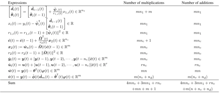
is a large dimension informational matrix, which gives rise to heavy computational burden. Differing from the M-GESG algorithm, the F-PC-GESG algorithm in (23)–(41) divides the system in (1) into one noise model andmfiltered subsystems. Moreover, the F-PC-GESG algorithm uses the data filtering to reduce the influence of the noise and improve the estimation accuracy. For everyt, the F-PC-GESG algorithm first gets the noise parameter vectorcˆ(t), and uses it to calculate the filtered input and output, then identifies the param-etersθˆi(t)anddˆi(t)based on the coupled relations between these filtered subsystems. This property also can be seen in Figure 1. Remark 7: The computational efficiency of an algorithm can be measured by using flops. The computational costs of the M-GESG algorithm and the F-PC-GESG algorithm are listed in Tables 1–2, wheren0=nc+nd+mn, n1=n+nd and n=mna+rnb. In order to make it clear, we take an example. Assume thatm= 10,
r= 10,na= 10, nb= 10,nc= 10and nd= 10. Then we can calculate N1−N2= 167630−17811 = 149819. It shows that
the F-PC-GESG algorithm has a higher computational efficiency than the M-GESG algorithm. For the system with high orders, the advantage of the F-PC-GESG algorithm becomes more obvious.
The proposed algorithms in this paper can be developed to mul-tivariable bilinear systems with colored noises [36–38], and can combine the neural network methods [39] and the kernel meth-ods [40, 41] to study parameter identification of different systems [42–44].
5 Examples
In this section, we give two numerical simulations to show the effectiveness of the proposed algorithm.
Example 1.Consider the following multivariable system with two-input two-output: A(z)y(t) =B(z)u(t) +D(z) C(z)v(t), A(z) =I2+ [ a11 a12 a21 a22 ] z−1 = [ 1 + 0.24z−1 0.94z−1 −0.80z−1 1 + 1.05z−1 ] , B(z) = [ b11 b12 b21 b22 ] z−1= [ 0.10z−1 0.15z−1 0.12z−1 −0.10z−1 ] , C(z) = 1 +c1z−1= 1 + 0.14z−1, D(z) = 1 +d1z−1= 1−0.80z−1, θT= [ 0.24 0.94 0.10 0.15 −0.80 1.05 0.12 −0.10 ] , ρ= [c1, d1]T= [0.14,−0.80]T, ϑ= [ ρ col[θT] ] .
To apply the proposed method, it is necessary to collect the input and output data. Here, we take the inputs {u1(t)} and {u2(t)} as two
independent persistent excitation signal sequences with zero mean and unit variances, and {v1(t)} and {v2(t)} are taken as two white
noise sequences with zero mean and variancesσ21=0.202forv1(t)
and σ22=0.302forv2(t). Then, we can compute the output vector y(t) = [y1(t), y2(t)]Tbased on the given input signals, the model
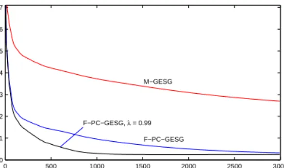
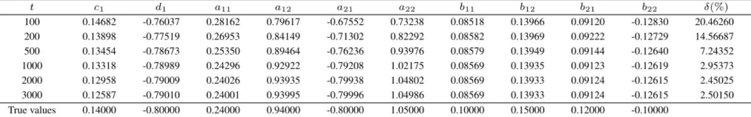
and the simulation condition. After obtaining the input and output data, apply the M-GESG algorithm in (45)–(52) and the F-PC-GESG algorithm in (23)–(41) to estimate the parameters of this system. In addition, we add a forgetting factorλ= 0.99to the F-PC-GESG algorithm to estimate the parameters. The parameter estimates and errors are shown in Tables 3–5. The parameter estimation errorsδ:=
∥ϑˆ(t)−ϑ∥/∥ϑ∥versustand the parameter estimates versustare
shown in Figure 2–4. 0 500 1000 1500 2000 2500 3000 0 0.1 0.2 0.3 0.4 0.5 0.6 0.7 M−GESG F−PC−GESG F−PC−GESG, λ = 0.99 t δ
Fig. 2: The parameter estimation errors versust
0 500 1000 1500 2000 2500 3000 −0.8 −0.6 −0.4 −0.2 0 0.2 0.4 0.6 0.8 1 1.2 t Parameter estimates c 1 d1 a 11 a21 b 22
Fig. 3: The M-GESG parameter estimates ˆc1(t), dˆ1(t), ˆa11(t), ˆ a21(t),ˆb22(t)versust 0 500 1000 1500 2000 2500 3000 −0.8 −0.6 −0.4 −0.2 0 0.2 0.4 0.6 0.8 1 1.2 t Parameter estimates c 1 d 1 a11 a21 b22
Fig. 4: The F-PC-GESG parameter estimatesˆc1(t),dˆ1(t),ˆa11(t), ˆ
Table 1 The computational efficiency of the M-GESG algorithm
Expressions Number of multiplications Number of additions
ˆ ϑ(t) = ˆϑ(t−1) + ˆ ΦT(t) r(t) e(t)∈R n0 mn 0+m mn0 e(t) :=y(t)−Φˆ(t) ˆϑ(t−1)∈Rm mn0 mn0 r(t) =r(t−1) +∥Φˆ(t)∥2∈R mn0 mn0 ˆ Φ(t) = [ ˆψ(t),φT(t)⊗I m]∈Rm×n0 n ˆ w(t) =y(t)−θT(t)φ(t)∈Rm mn mn ˆ v(t) =y(t)−Φˆ(t) ˆϑ(t)∈Rm mn0 mn0 Sum 4mn0+mn+m+n 4mn0+mn Total flops N1= 8mn0+ 2mn+m+n
Table 2 The computational efficiency of the F-PC-GESG algorithm
Expressions Number of multiplications Number of additions
[ ˆ di(t) ˆ θi(t) ] = [ ˆ di−1(t) ˆ θi(t−1) ] + ˆ ψi(t) r1,i(t)x1,i(t)∈R n1 mn 1+m mn1 xi(t) :=yi(t)−ψˆ T i(t) [ ˆ di−1(t) ˆ θi(t−1) ] ∈R mn1 mn1 r1,i(t) =r1,i(t−1) +∥ψˆi(t)∥2∈R mn1 mn1 ˆ c(t) = ˆc(t−1) +Ωˆ T (t) r2(t) x2(t)∈R nc mn c+ 1 mnc x2(t) := ˆwn(t)−Ωˆ(t)ˆc(t−1)∈Rm mnc mnc r2(t) =r2(t−1) +∥Ωˆ(t)∥2∈R mnc mnc ˆ yf(t) =y(t) + [y(t−1),y(t−2),· · ·,y(t−nc)]ˆc(t)∈Rm mnc mnc ˆ uf(t) =u(t) + [u(t−1),u(t−2),· · ·,u(t−nc)]ˆc(t)∈Rr rnc rnc ˆ w(t) =y(t)−θT(t)φ(t)∈Rm mn mn ˆ v(t) =y(t)−ϕˆ(t) ˆdm(t)−θˆ T (t)φ(t)∈Rm m(nc+nd) m(nc+nd) Sum 4mnc+ 3mn1+rnc 4mnc+ 3mn1+rnc +mn+m+ 1 +m(n+nc+nd) Total flops N2= 9mnc+ 6mn1+ 2rnc+m(2n+nd) +m+ 1
Table 3 The M-GESG parameter estimates and errors
t c1 d1 a11 a12 a21 a22 b11 b12 b21 b22 δ(%) 100 0.29814 -0.37722 0.17325 0.60704 -0.44106 0.39523 0.09329 0.19856 0.15585 0.14712 52.61754 200 0.31325 -0.41248 0.18312 0.67058 -0.51004 0.44544 0.09371 0.19839 0.15499 0.14735 47.59884 500 0.32579 -0.44659 0.19271 0.73519 -0.58466 0.51074 0.09380 0.19812 0.15509 0.14702 42.19534 1000 0.33453 -0.47454 0.20027 0.79069 -0.65147 0.58459 0.09380 0.19811 0.15518 0.14697 37.21425 2000 0.34254 -0.50497 0.21045 0.85604 -0.72945 0.70419 0.09378 0.19812 0.15511 0.14698 30.92303 3000 0.34628 -0.52138 0.21874 0.89587 -0.77404 0.80734 0.09378 0.19812 0.15511 0.14698 26.93724 True values 0.14000 -0.80000 0.24000 0.94000 -0.80000 1.05000 0.10000 0.15000 0.12000 -0.10000
Table 4 The F-PC-GESG parameter estimates and errors
t c1 d1 a11 a12 a21 a22 b11 b12 b21 b22 δ(%) 100 0.14689 -0.75226 0.28804 0.77230 -0.65336 0.68846 0.08574 0.13932 0.09144 -0.13092 23.45508 200 0.13990 -0.76652 0.27860 0.80983 -0.68485 0.75869 0.08627 0.13935 0.09232 -0.13025 18.75964 500 0.13497 -0.77753 0.26826 0.84469 -0.71807 0.82916 0.08624 0.13931 0.09195 -0.12974 14.12815 1000 0.13303 -0.78535 0.25797 0.87810 -0.74940 0.90104 0.08616 0.13928 0.09178 -0.12966 9.57124 2000 0.13030 -0.79015 0.24796 0.91167 -0.77756 0.97892 0.08617 0.13927 0.09181 -0.12965 5.02683 3000 0.12748 -0.79124 0.24341 0.92736 -0.78984 1.01712 0.08617 0.13927 0.09181 -0.12965 3.23992 True values 0.14000 -0.80000 0.24000 0.94000 -0.80000 1.05000 0.10000 0.15000 0.12000 -0.10000
Example 2.Consider the following multivariable system:
A(z)y(t) =B(z)u(t) +d(z) c(z)v(t), A(z) =I3+ aa14 aa25 aa36 a7 a8 a9 z−1 = −−00..5563 −00..6445 −00..1556 0.69 0.32 −0.41 z−1, B(z) = bb14 bb25 bb36 b7 b8 b9 z−1 = 00..1310 −−00..0808 −−00..1320 −0.09 0.07 0.17 z−1, c(z) = 1 +c1z−1= 1−0.73z−1, d(z) = 1 +d1z−1= 1 + 0.68z−1, ρT= −−00..5563 −00..6445 −00..5615 00..1013 −−00..0808 −−00..1320 0.69 0.32 −0.41 −0.09 0.07 0.17 , β= [c , d ]T= [−0.73,0.68]T,
Here, we take the inputs {u1(t)}, {u2(t)} and {u3(t)} as three
independent persistent excitation signal sequences with zero mean and unit variances, and {v1(t)}, {v2(t)} and {v3(t)} are taken
as three white noise sequences with zero mean and variances
σ12=σ22=σ23=0.102forv1(t),v2(t)andv3(t). We use the M-GESG
algorithm and the PC-GESG algorithm to estimate the parameters of this multivariable system, respectively. Since there are 20 param-eters, we do not give the table for parameter estimates and errors.
IET Research Journals,pp. 1–9 c
Table 5 The F-PC-GESG parameter estimates and errors (λ= 0.99) t c1 d1 a11 a12 a21 a22 b11 b12 b21 b22 δ(%) 100 0.14682 -0.76037 0.28162 0.79617 -0.67552 0.73238 0.08518 0.13966 0.09120 -0.12830 20.46260 200 0.13898 -0.77519 0.26953 0.84149 -0.71302 0.82292 0.08582 0.13969 0.09222 -0.12729 14.56687 500 0.13454 -0.78673 0.25350 0.89464 -0.76236 0.93976 0.08579 0.13949 0.09144 -0.12640 7.24352 1000 0.13318 -0.78989 0.24296 0.92922 -0.79208 1.02175 0.08569 0.13935 0.09123 -0.12619 2.95373 2000 0.12958 -0.79009 0.24026 0.93935 -0.79938 1.04802 0.08569 0.13933 0.09124 -0.12615 2.45025 3000 0.12587 -0.79010 0.24001 0.93995 -0.79996 1.04986 0.08569 0.13933 0.09124 -0.12615 2.50150 True values 0.14000 -0.80000 0.24000 0.94000 -0.80000 1.05000 0.10000 0.15000 0.12000 -0.10000
Here, we use the parameter estimation errors curve to show the per-formance of the algorithms. The parameter estimation errors versus
tare shown in Figure 5.
0 500 1000 1500 2000 2500 3000 0 0.1 0.2 0.3 0.4 0.5 0.6 0.7 M−GESG F−PC−GESG t δ
Fig. 5: The parameter estimation errors versust
From Tables 3–5 and Figures 2–5, we can draw the following conclusions.
1. The parameter estimation errors of the M-GESG and the F-PC-GESG algorithms become smaller with the data lengthtincreasing – see the estimation errors of the last columns in Tables 3–5. 2. Under the same noise level, the PC-GESG algorithm has a higher parameter estimation accuracy than the M-GESG algorithm – see Tables 3–5 and Figures 2–4. This demonstrates that the proposed algorithm is effective.
3. Introducing a forgetting factor can improve the parameter esti-mation accuracy of the F-PC-GESG algorithm – see Table 5 and Figure 2.
6 Conclusions
In this paper, the parameter estimation problem has been investigated for multivariable CARARMA systems. An F-PC-GESG algorithm is derived by adopting the filtering technique and the coupling concept. In order to reduce the influence of the noise, we construct a filter to filter the input and output data and transform the system into two parts, including a noise model and a filtered system model. In addi-tion, the filtered system model is divided into several subsystems and identified by the coupling concept. According to the computational comparison, the F-PC-GESG algorithm has less computational bur-den than the M-GESG algorithm. The simulation results indicate that the F-PC-GESG algorithm can generate more accurate parameter estimates. Moreover, introducing the forgetting factor can improve the performance of the F-PC-GESG algorithm. The basic idea of the proposed method in this paper can be used to study the parameter identification problems of other multivariable systems with different structures and disturbance noises.
The identification method presented in this paper can combine the multi-innovation methods [45] and some mathematical skills [46–48] and statistical methods [49–51] can be used to study the performances of parameter estimation algorithms and can be applied other fields [52–55].
7 Acknowledgments
This work was supported by the National Natural Science Foun-dation of China (grant no. 61873111), the 111 Project (grant no. B12018) and the National First-Class Discipline Program of Light Industry Technology and Engineering (grant no. LITE2018-26).
8 References
1 Cao, Y., Li, P., Zhang, Y.: ‘Parallel processing algorithm for railway signal fault diagnosis data based on cloud computing’,Future Generation Computer Systems, 2018,88, pp. 279-283
2 Zhou, Z.P., Liu, X.F.: ‘State and fault estimation of sandwich systems with hys-teresis’,International Journal of Robust and Nonlinear Control, 2018,28, (13), pp. 3974-3986
3 Cao, Y., Ma, L.C., Xiao, S.,et al.: ‘Standard analysis for transfer delay in CTCS-3’,
Chinese Journal of Electronics, 2017,26, (5), pp. 1057-1063
4 Zhang, Y.Z., Cao, Y., Wen, Y.H.,et al.: ‘Optimization of information interac-tion protocols in cooperative vehicle-infrastructure systems’,Chinese Journal of
Electronics, 2018,27, (2), pp. 439-444
5 Cao, Y., Ma, L.C., Xiao, S.,et al.: ‘Standard analysis for transfer delay in CTCS-3’,
Chinese Journal of Electronics, 2017,26, (5), pp. 1057-1063
6 Wang, Y., Zhang, H., Wei, S., et al.: ‘Control performance assessment for ILC-controlled batch processes in two-dimensional system framework’,IEEE
Transactions on Systems, Man, and Cybernetics: Systems, 2018, 48, (9), pp.
1493-1504
7 Zhang, W.H., Xue, L., Jiang, X.: ‘Global stabilization for a class of stochastic nonlinear systems with SISS-like conditions and time delay’,International Journal
of Robust and Nonlinear Control, 2018,28, (13), pp. 3909-3926
8 Xu, L.: ‘The parameter estimation algorithms based on the dynamical response measurement data’,Advances in Mechanical Engineering, 2017,9, (11), pp. 1-12, doi: 10.1177/1687814017730003
9 Xu, L., Ding, F.: ‘Iterative parameter estimation for signal models based on measured data’, Circuits Systems and Signal Processing, 2018, 37, (7), pp. 3046-3069
10 Dong, S.J., Liu, T., Wang, Q.G.: ‘Identification of dual-rate sampled systems with time delay subject to load disturbance’,IET Control Theory and Applications, 2017,11, (9), pp. 1404-1413
11 Na, J., Yang, J., Wu, X.,et al.: ‘Robust adaptive parameter estimation of sinusoidal signals’,Automatica, 2015,53, pp. 376-384
12 Xu, L., Ding, F.: ‘Parameter estimation for control systems based on impulse responses’,International Journal of Control, Automation, and Systems, 2017,15, (6), pp. 2471-2479
13 Bottegal, G., Aravkin, A.Y., Hjalmarsson, H., Pillonetto, G.: ‘Robust EM kernel-based methods for linear system identification’,Automatica, 2016,67, pp. 114-126 14 Gan, M., Chen, C.L.P., Chen, G.Y., Chen, L: ‘On some separated algorithms for separable nonlinear squares problems’,IEEE Transactions on Cybernetics, 2018,
48, (10), pp. 2866-2874
15 Na, J., Yang, J., Ren, X.M.,et al.: ‘Robust adaptive estimation of nonlinear sys-tem with time-varying parameters’,International Journal of Adaptive Control and
Signal Processing, 2015,29, (8), pp. 1055-1072
16 Mattsson, P., Zachariah, D., Stoica, P.: ‘Recursive nonlinear-system identification using latent variables’,Automatica, 2018,93, pp. 343-351
17 Li, J.H., Zheng, W.X., Gu, J.P., Hua, L.: ‘A recursive identification algorithm for Wiener nonlinear systems with linear state-space subsystem’,Circuits Systems and
Signal Processing, 2018,37, (6), pp. 2374-2393
18 Doraiswami, R., Cheded, L.: ‘Robust Kalman filter-based least squares identifica-tion of a multivariable system’,IET Control Theory and Applications, 2018,12, (8), pp. 1064-1074
19 Gan, M., Li, H.X., Peng, H.: ‘A variable projection approach for efficient estima-tion of RBF-ARX model’,IEEE Transactions on Cybernetics, 2015,45, (3) pp. 462-471
20 Yu, C.P., Verhaegen, M.: ‘Blind multivariable ARMA subspace identification’,
Automatica, 2016,66, pp. 3-14
21 Cham, C.L., Tan, A.H., Tan, W.H.: ‘Identification of a multivariable nonlinear and time-varying mist reactor system’,Control Engineering Practice, 2017,63, pp. 13-23
22 Ding, S., Dang, Y.G., Li, X.M.,et al.: ‘Forecasting ChineseCO2emissions from
fuel combustion using a novel grey multivariable model’,Journal of Cleaner
Production, 2017,162, pp. 1527-1538
23 Mobayen, S.: ‘Robust tracking controller for multivariable delayed systems with input saturation via composite nonlinear feedback’,Nonlinear Dynamics, 2014,
24 Zhang, E.L., Pintelon, R.: ‘Identification of multivariable dynamic errors-in-variables system with arbitrary inputs’,Automatica, 2017,82, pp. 69-78 25 Ding, J.L.: ‘Recursive and iterative least squares parameter estimation
algo-rithms for multiple-input-output-error systems with autoregressive noise’,Circuits
Systems and Signal Processing, 2018,37, (5), pp. 1884-1906
26 Li, M.H., Liu, X.M.: ‘The least squares based iterative algorithms for parameter estimation of a bilinear system with autoregressive noise using the data filtering technique’,Signal Processing, 2018,147, pp. 23-34
27 Pan, J., Ma, H., Jiang, X., et al.: ‘Adaptive gradient-based iterative algorithm for multivariate controlled autoregressive moving average systems using the data filtering technique’, Complexity, 2018, Article ID 9598307. https://doi.org/10.1155/2018/9598307
28 Afshari, H.H., Gadsden, S.A., Habibi, S.: ‘Gaussian filters for parameter and state estimation: A general review of theory and recent trends’,Signal Processing, 2017,
135, pp. 218-238
29 Pan, J., Jiang, X., Wan, X.K., Ding, W.F.: ‘A filtering based multi-innovation extended stochastic gradient algorithm for multivariable control systems’,
Interna-tional Journal of Control, Automation, and Systems, 2017,15, (3), pp. 1189-1197
30 Xu, L., Xiong, W.L., Alsaedi, A., Hayat, T.: ‘Hierarchical parameter estimation for the frequency response based on the dynamical window data’,International
Journal of Control, Automation and Systems,2018,16, (4), pp. 1756-1764
31 Ding, J.L.: ‘The hierarchical iterative identification algorithm for multi-input-output-error systems with autoregressive noise’,Complexity, 2017, pp. 1-11. Article ID 5292894. https://doi.org/10.1155/2017/5292894
32 Ding, F.: ‘Coupled-least-squares identification for multivariable systems’,IET
Control Theory and Applications, 2013,7, (1), pp. 68-79
33 Ding, F., Liu, G., Liu, X.P.: ‘Partially coupled stochastic gradient identification methods for non-uniformly sampled systems’,IEEE Transactions on Automatic
Control, 2010,55, (8), pp. 1976-1981
34 Wang, X.H., Ding, F.: ‘Partially coupled extended stochastic gradient algorithm for nonlinear multivariable output error moving average systems’,Engineering
Computations, 2017,34, (2), pp. 629-647
35 Liu, Q.Y., Ding, F., Yang, E.F.: ‘Parameter estimation algorithm for multivariable controlled autoregressive autoregressive moving average systems’,Digital Signal
Processing, 2018,83, pp. 323-331
36 Zhang, X., Xu, L., Ding, F.,et al.: ‘Combined state and parameter estimation for a bilinear state space system with moving average noise’,J. Franklin Inst., 2018,
355, (6), pp. 3079-3103.
37 Zhang, X., Ding, F., Xu, L.,et al.: ‘State filtering-based least squares parameter estimation for bilinear systems using the hierarchical identification principle’,IET
Control Theory Appl., 2018,12, (12), pp. 1704-1713.
38 Zhang, X., Ding, F., Alsaadi, F.E., Hayat, T.: ‘Recursive parameter identification of the dynamical models for bilinear state space systems’,Nonlinear Dyn., 2017,
89, (4), pp. 2415-2429
39 Li, X., Zhu, D.Q. : ’An improved SOM neural network method to adaptive leader-follower formation control of AUVs’,IEEE Transactions on Industrial Electronics, 2018,65, (10), pp. 8260-8270
40 Geng, F.Z., Qian, S.P.: ‘An optimal reproducing kernel method for linear nonlocal boundary value problems’,Appl. Math. Lett., 2018,77, pp. 49-56.
41 Li, X.Y., Wu, B.Y.: ‘A new reproducing kernel collocation method for nonlocal fractional boundary value problems with non-smooth solutions’,Appl. Math. Lett., 2018,86, pp. 194-199. December ´s˙zÒýˇcž0
42 Ding, F., Xu, L., Alsaadi, F.E.,et al.: ‘Iterative parameter identification for pseudo-linear systems with ARMA noise using the filtering technique’, IET Control
Theory Appl., 2018,12, (7), pp. 892-899.
43 Ding, F., Chen, H.B., Xu, L.,et al.: Dai, J.Y., Li, Q.S., Hayat, T.: ‘A hierarchical least squares identification algorithm for Hammerstein nonlinear systems using the key term separation’,J. Franklin Inst., 2018,355, (8), pp. 3737-3752.
44 Wang, Y.J., Ding, F., Xu, L.: ‘Some new results of designing an IIR filter with colored noise for signal processing’,Digit. Signal Process., 2018,72, pp. 44-58 45 Ding, F.: ‘Several multi-innovation identification methods’,Digital Signal
Pro-cessing,20, (4), pp. (2010) 1027-1039.
46 Liu, F., Wu, H.X.: ‘Singular integrals related to homogeneous mappings in triebel-lizorkin spaces’,Journal of Mathematical Inequalities, 2017,11, (4), pp. 1075-1097 Cited 12
47 Liu, F., Wu, H.X.: ‘Regularity of discrete multisublinear fractional maximal functions’,Science China – Mathematics, 2017,60, (8), pp. 1461-1476 Cited 14 48 Liu, F., Wu, H.X.: ‘On the regularity of maximal operators supported by
subman-ifolds’,Journal of Mathematical Analysis and Applications, 2017,453, (1), pp. 144-158 Cited 13
49 Yin, C.C., Wen, Y.Z.: ‘Exit problems for jump processes with applications to dividend problems’,J. Comput. Appl. Math., 2013,245, pp. 30-52
50 Yin, C.C., Wen, Y.Z.: ‘Optimal dividend problem with a terminal value for spec-trally positive Levy processes’,Insurance Mathematics & Economics, 2013,53, (3), pp. 769-773
51 Yin, C.C., Wang, C.W.: ‘The perturbed compound Poisson risk process with invest-ment and debit interest’,Methodology and Computing in Applied Probability, 2010,12, (3), pp. 391-413
52 Gong, P.C., Wang, W.Q., Li, F.C., Cheung, H.: ‘Sparsity-aware transmit beamspace design for FDA-MIMO radar’,Signal Process., 2018,144, pp. 99-103. 53 Rao, Z.H., Zeng, C.Y., Wu, M.H. Wu, et al.: ‘Research on a handwritten character
recognition algorithm based on an extended nonlinear kernel residual network’,
KSII Transactions on Internet and Information Systems, 2018,12, (1), pp. 413-435.
54 Zhao, N., Liu, R., Chen, Y., Wu, M., et al.: ‘Contract design for relay incentive mechanism under dual asymmetric information in cooperative networks’,Wireless
Networks, 2018,24, (8), pp. 3029-3044.
55 Pan, J., Li, W., Zhang, H.P.: ‘Control algorithms of magnetic suspension sys-tems based on the improved double exponential reaching law of sliding mode control’, International Journal of Control, Automation and Systems, 2018.