O R I G I N A L A R T I C L E
Open Access
Optimization of underwater wet welding process
parameters using neural network
Joshua Emuejevoke Omajene
*, Jukka Martikainen, Huapeng Wu and Paul Kah
Abstract
Background:The structural integrity of welds carried out in underwater wet environment is very key to the reliability of welded structures in the offshore environment. The soundness of a weld can be predicted from the weld bead geometry.
Methods:This paper illustrates the application of artificial neural network approach in the optimization of the welding process parameter and the influence of the water environment. Neural network learning algorithm is the method used to control the welding current, voltage, contact tube-to-work distance, and speed so as to alter the influence of the water depth and water environment.
Results:The result of this work gives a clear insight of achieving proper weld bead width (W), penetration (P), and reinforcement (R).
Conclusions:An interesting implication of this work is that it will lead to a robust welding activity so as to achieve sound welds for offshore construction industries.
Keywords:Backpropagation; Bead geometry; Neural network; Process parameter; Underwater welding
Background
The differences in the weld quality for underwater weld-ing as compared to air weldweld-ing have made it very neces-sary to model an artificial neural network (ANN) which is capable of solving difficult and complex problems. The weld bead geometry of an underwater wet welding can be predicted by the neural network control of the input parameters as shown in Figure 1. The water sur-rounding the weld metal results in a fast cooling of the weld, thereby reducing the ductility and tensile strength of the weld metal by 50% and 20%, respectively (Brown and Masubuchi 1975). The effect of the water environment and the water depth on the welding process parameters significantly affects the quality of welds achieved under-water. The diffusible hydrogen contents are increased at lower water temperature for lower oxygen content. The in-crease in the diffusible hydrogen content leads to inin-crease in the susceptibility of steels to hydrogen-assisted cracking (Johnson 1997). The water depth plays a role in the stabil-ity of the welding arc. Increased water depth constricts the
arc, thereby resulting in an increased current and voltage as the water depth increases. An increasing water depth decreases the operating process parameter space (Liu et al. 1993). This paper proposes suitable means of optimizing the welding process parameter using a neural network so as to minimize the effect of the cooling rate and water depth in underwater welding. The main goal is to achieve a weld bead geometry which will give the weld metal the recommended structural integrity as pre-scribed by the underwater welding specification code AWS D3.6M:2010 (AWS 2010).
Methods
Underwater welding
Underwater welding is used for the repair welding of ships and offshore engineering structures like oil drilling rigs, pipelines, and platforms. The commonly used underwater welding processes nowadays are shielded metal arc welding (SMAW) and flux cored arc welding (FCAW). The water surrounding the weld metal reduces the mechanical prop-erties of weld done underwater due to the effect of the fast cooling rate of the weld. Heat loss by conduction from the * Correspondence:[email protected]
LUT Mechanical Engineering, Lappeenranta University of Technology, P.O. Box 20, FI-53851 Lappeenranta, Finland
plate surface into the moving water environment and heat loss by radiation are the major heat losses in underwater welding. Underwater welding requires a higher current for the same arc voltage to achieve a higher heat input as com-pared to air welding. The fast cooling rate of underwater welding results in the formation of constituents such as martensite and bainite for conventional welding of steels. These constituents lead to a high-strength, brittle material and susceptibility to hydrogen-induced cracking. The weld bead shape for underwater wet welding are more spread out and less penetrating than air welds. Underwater weld-ing arc is constricted at increased depth or pressure. How-ever, welding in shallow depth is more critical than that in higher depth. The unstable arc results in porosity which affects the soundness of the weld. Weld metal carbon
content increases with increase in water depth. Also, man-ganese and silicon which are deoxidizers are increasingly lost at increased water depth (Omajene et al. 2014).
Artificial neural network
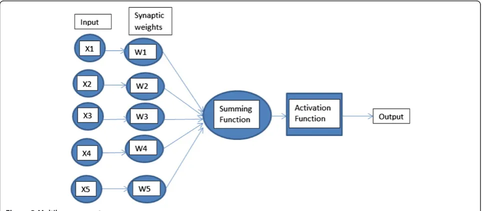
A neural network is a data modeling tool that captures and represents complex input/output relationships. A neuron gets signals from its input links, computes a new activation level, and sends an output signal through the output link(s). The learning algorithm is the procedure to modify the synaptic weights of the network to achieve the desired objective of the design. Weights are the basic means of long-term memory in artificial neural net-works. The multilayer perceptron neural network (NN) is the most applicable network architecture in use today. Figure 1Welding input vs output parameters.
Each unit as shown in Figure 2 undergoes a biased weighted sum of its inputs and passes it through an activa-tion funcactiva-tion to produce its output. These units are ar-ranged in a layered feed forward topology. The multilayer perceptron neural network learns using backpropagation algorithm as shown in Figure 3. In backpropagation algo-rithm, the input data is repeatedly presented to the neural network. In each presentation, the output of the neural network is compared to the desired output, thereby com-puting an error signal. The error is presented back to the neural network to adjust the weights in a manner that the error decreases with each iteration and the neural network model gets closer to the desired target. Figure 3 illustrates a neural network using the backpropagation algorithm whereby the weight is changed as the iteration increases,
thereby reducing the error and getting closer to the de-sired target (Al-Faruk et al. 2010; Juang et al. 1998).
Summary of the backpropagation training algorithm The summary of the backpropagation training algorithm is illustrated as follows (Negnevetsky 2005).
Step 1: Initialization
−2:4
Fi ;þ 2:4
Fi
Set the weights and threshold levels of the network to uniformly random numbers distributed in small range.Fi is the total number of inputs of neuroniin the network. Figure 3Three-layer backpropagation neural network (Negnevetsky 2005).
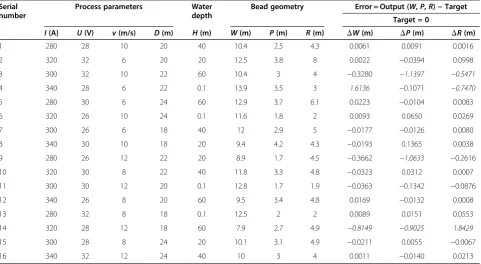
Table 1 Experimental data adapted from (Shi et al. 2013)
Serial number
Process parameters Water
depth
Bead geometry Error = Output (W,P,R)−Target
Target = 0
I(A) U(V) v(m/s) D(m) H(m) W(m) P(m) R(m) ΔW(m) ΔP(m) ΔR(m)
1 280 28 10 20 40 10.4 2.5 4.3 0.0061 0.0091 0.0016
2 320 32 6 20 20 12.5 3.8 8 0.0022 −0.0394 0.0998
3 300 32 10 22 60 10.4 3 4 −0.3280 −1.1397 −0.5471
4 340 28 6 22 0.1 13.9 3.5 3 1.6136 −0.1071 −0.7470
5 280 30 6 24 60 12.9 3.7 6.1 0.0223 −0.0104 0.0083
6 320 26 10 24 0.1 11.6 1.8 2 0.0093 0.0650 0.0269
7 300 26 6 18 40 12 2.9 5 −0.0177 −0.0126 0.0080
8 340 30 10 18 20 9.4 4.2 4.3 −0.0193 0.1365 0.0038
9 280 26 12 22 20 8.9 1.7 4.5 −0.3662 −1.0633 −0.2616
10 320 30 8 22 40 11.8 3.3 4.8 −0.0323 0.0312 0.0007
11 300 30 12 20 0.1 12.8 1.7 1.9 −0.0363 −0.1342 −0.0876
12 340 26 8 20 60 9.5 3.4 4.8 0.0169 −0.0132 0.0008
13 280 32 8 18 0.1 12.5 2 2 0.0089 0.0151 0.0553
14 320 28 12 18 60 7.9 2.7 4.9 −0.8149 −0.9025 1.8429
15 300 28 8 24 20 10.1 3.1 4.9 −0.0211 0.0055 −0.0067
Step 2: Activation
Activate the backpropagation neural network by apply-ing inputsx1(p),x2(p),…,xn(p) and desired outputyd,1(p),
yd,2(p),…,yd,n(p).
(a) Calculate the actual outputs of the neurons in the hidden layer:
yjð Þ ¼p sigmoid Xn
i¼0xið Þ p wijð Þp −θj
h i
wherenis the number of inputs of neuronjin the hidden layer and sigmoid is the sigmoid activation function.
(b)Calculate the actual outputs of the neurons in the output layer.
(c)ykð Þ ¼p sigmoid Xm
j¼0yjð Þ p wjkð Þp −θk
h i
wheremis the number of inputs of neuronkin the out-put layer.
Step 3: Weight training
Update the weights in the backpropagation network propagating backward the errors associated with output neurons.
(a) Calculate the error gradient for the neurons in the output layer:
δkð Þ ¼p ykð Þ p 1–ykð Þp
ekð Þp
where
ekð Þ ¼p yd;kð Þp –ykð Þp
Calculate the weight corrections
Δwjkð Þ ¼p αyjð Þ p δkð Þp
Update the weights at the output neurons:
wjkðpþ1Þ ¼wjkð Þ þp Δwjkð Þp
(b)Calculate the error gradient for the neurons in the hidden layer:
δjð Þ ¼p yjð Þ p 1–yjð Þp
h i
Xℓk¼0δkð Þ p wjkð Þp
Calculate the weight corrections
Δwijð Þ ¼p αxið Þ p δjð Þp
Update the weights at the output neurons:
wijðpþ1Þ ¼wijð Þ þp Δwijð Þp
Step 4: Increase iterationpby 1, go back to step 2, and repeat the process until the selected error criterion is satisfied.
Results and discussion
The ANN scheme to predict the weld bead geometry in underwater wet welding is shown in Figure 1. The aim is to map a set of input patterns to a corresponding set of output patterns by learning from past examples how the input parameters and output parameters relate. A feed-forward backpropagation network trained with scaled conjugate gradient (SCG) backpropagation algorithm is used. The quality of the weld can be verified when the training pattern fulfills the requirement for the accepted
ranges of WPSF (penetration shape factor) =W/P and
WRFF (reinforcement form factor) =W/R. The accepted ranges for a weld with good quality are a maximized penetration to width ratio and minimized undercut and reinforcement.
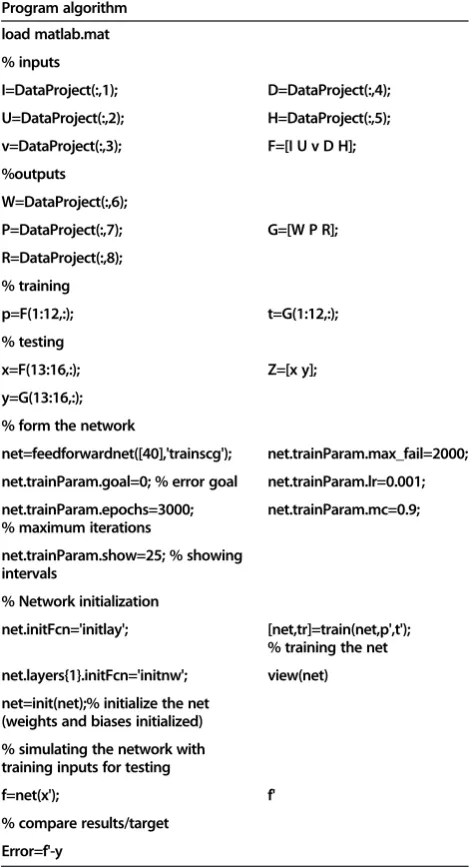
Table 2 Program algorithm
Program algorithm
load matlab.mat
% inputs
I=DataProject(:,1); D=DataProject(:,4);
U=DataProject(:,2); H=DataProject(:,5);
v=DataProject(:,3); F=[I U v D H];
%outputs
W=DataProject(:,6);
P=DataProject(:,7); G=[W P R];
R=DataProject(:,8);
% training
p=F(1:12,:); t=G(1:12,:);
% testing
x=F(13:16,:); Z=[x y];
y=G(13:16,:);
% form the network
net=feedforwardnet([40],'trainscg'); net.trainParam.max_fail=2000;
net.trainParam.goal=0; % error goal net.trainParam.lr=0.001;
net.trainParam.epochs=3000; % maximum iterations
net.trainParam.mc=0.9;
net.trainParam.show=25; % showing intervals
% Network initialization
net.initFcn='initlay'; [net,tr]=train(net,p',t');
% training the net
net.layers{1}.initFcn='initnw'; view(net)
net=init(net);% initialize the net (weights and biases initialized)
% simulating the network with training inputs for testing
f=net(x'); f'
% compare results/target
Design parameters
The experimental data values in Table 1 for process parameters, water depth and bead geometry are the values used for the training of) the neural network. These values are from an experimental data adapted from the work of Shi et al. (2013). The error results for each testing are included in the modified table (Table 1). The errors in italics are the errors from the training which are big and not desirable. A smaller error tending to zero is desired or an actual zero which is however not so easy to achieve.
Program algorithm
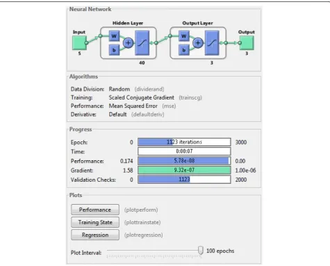
There are five input parameters and three output param-eters in this model (Table 2). The training (Figure 4) was done for all the sets of data, so also is the testing. The target is to achieve an error value of 0. The size of the hidden layer was obtained by iterative adjustment while measuring the error during the neural network testing (Nagendra & Khare 2006). The network for this study
has two layers; there are 40 neurons in the hidden layer. In this study, the neural network should ideally be able to learn and understand the interaction between the welding process parameters. There are different training algorithms for different processes. The SCG backpropagation algo-rithm was used for the training of the network because it is suitable for the training of larger networks. Other training algorithms had the problem of overfitting caused by over-training, resulting in memorization of input/output instead of analyzing them on the internal factors determined by the updated weights. The learning rate used is 0.001 and it gave satisfactory results. In artificial neural networks, a high learning rate may lead to overshooting, while a slow learn-ing rate takes more time for the network to converge.
Validation performance
Epoch is a single presentation of each input/output data on the training set. It indicates the iteration at which the validation performance reached a minimum (Fahlman
0 200 400 600 800 1000 10-8
10-6 10-4 10-2 100
Best Validation Performance is 0.00091499 at epoch 0
M
e
a
n
S
q
ua
re
d
E
rr
or
(m
s
e
)
1123 Epochs
Train Validation Test Best
Figure 5Validation performance curve.
1988). The training continued for 1,123 more iteration before the training stopped. Figure 5 does not indicate any major problems with the training. The validation and test curve are very similar. If the curve had creased significantly before the validation curve in-creases, then it is possible that some overfitting might have occurred. The final mean squared error (MSE) is
small, which is 9.1499e−4 at zero epoch. The MSE is
used to gauge the performance of the network. The MSE is an average of the squares of all the individual er-rors between the model and the real measurements. The MSE is useful for comparing different models with the same sets of data.
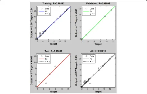
Regression analysis
This plot is used to validate the network performance. The regression plots in Figure 6 display the network out-puts with respect to targets for training, validation, and test sets. For a perfect fit, the network outputs are equal to the targets. The fit for this problem is reasonably good for all data sets withRvalues in each case at least 0.96637. These results are achieved by retraining which
changes the initial weights of the network. In this prob-lem, 100% of the data sets were used for training, valid-ation, and testing of the network generalization.
Controller for underwater wet welding process
Figure 7 is a proposed schematic diagram for a possible control of underwater wet welding in which the NN optimization of the welding process parameter can be applicable. The NN model in this paper will be an essen-tial part in the control architecture of the proposed con-troller with the aim of designing a robust concon-troller for underwater wet welding process, and further research work is necessary in this regard. The preliminary explan-ation of this possible controller is highlighted in this sec-tion. The control system is aimed at controlling the welding process parameters for different measured water depthH; the water depth is not a control parameter but a measured parameter as welding is being carried out at different water depth. The water depth for the welding process is measured as the depth changes. This change in the measured water depth consequently changes the welding process parameters which in turn alters the
bead geometry W, R, andP. The fuzzy controller com-pensates for this change and modifies the welding process parameters I, u,V, andD. The inverse NN has a constant parameter value which is the desired bead geometry parameter as inputs to the inverse NN and best parameter of the welding process as the output from the inverse NN. The error values for the training in experiment 1 from Table 1 are the best set of parame-ters because the errors forW,R, andPare closer to zero compared to the values for the other experiments. The constant output parametersI0,U0,v0,D0, andH0which is the water depth at zero position from the inverse NN are summed up with the difference from the change in the output parameters ΔI, ΔU, Δv, ΔD, respectively, of the fuzzy controller, and this compensates for the change in the welding process parameters and inputs the ad-justed welding process parameter to the welding ma-chine. For every measured change in the water depthH, a change in the bead geometryΔW,ΔP, andΔRwhich is the input to the fuzzy controller is modified and gives an output ofΔI, ΔU,Δv, andΔD. The welding process par-ameter from the welding machine is equal to the NN forward model, and as such, any change in the NN forward model is a subsequent change in the welding process itself. This control mechanism is a possible robust control process of the welding process and eliminates the need for online measurement of the weld bead geometry.
Conclusions
The optimization of the parameters that affect weld bead geometry during underwater welding can be done by artificial neural network training algorithm. In this study, the regression analysis show that the target follows closely the output asRis at least 96% for training, test-ing, and validation. The trained neural network with sat-isfactory results can be used as a black box in the control system of the welding process. The effective optimization of the welding process parameter in under-water wet welding has the ability of welding with an op-timized heat input and opop-timized arc length which will guarantee arc stability. The use of optimized process pa-rameters enables the achievement of an optimized weld bead geometry which is a key factor in the soundness of welds. The control process for underwater welding as suggested in this paper requires further research so as to fully apply the NN optimization process.
Competing interests
The authors declare that they have no competing interests.
Authors' contributions
The main author JEO carried out the research and designed the neural network model and analyzed the training results and prepared the paper. HW was responsible for key technical supervision. PK and JM checked the paper and provided suggestions to improve the paper. All authors read and approved the final manuscript.
Received: 8 September 2014 Accepted: 5 November 2014
References
Al-Faruk, A, Hasib, A, Ahmed, N, Kumar Das, U. (2010). Prediction of weld bead geometry and penetration in electric arc welding using artificial neural networks.International Journal of Mechanical & Mechatronics Engineering, 10 (4), 19–24.
AWS. (2010).“Underwater welding code”. USA: AWS.
Brown, RT, & Masubuchi, K. (1975).“Fundamental Research on Underwater Welding”. InWelding research supplement(pp. 178–188).
Fahlman, SE. (1988).An empirical study of learning speed in backpropagation. USA: Carnegie Mellon University.
Johnson, RL. (1997).The Effect of Water Temperature on Underbead Cracking of Underwater Wet Weldments. California: Naval Postgraduate School. Juang, SC, Tarng, YS, & Lii, HR. (1998). A comparison between the
backpropagation and counterpropagation networks in the modeling of TIG welding process.Journal of Material ocessing Technology, 75, 54–62. Liu, S, Olson, DL, & Ibarra, S. (1993). Underwater Welding.ASM Handbook, 6,
1010–1015.
Nagendra, SM, & Khare, M. (2006). Artificial neural network approach for modelling nitrogen dioxide dispersion from vehicular exhaust emissions. Ecological Modelling, 190(1–2), 99–115.
Negnevetsky, M. (2005).Artificial Intelligence. UK: Addison Wesley.
Omajene, JE, Martikainen, J, Kah, P, & Pirinen, M. (2014). Fundamental difficulties associated with underwater wet welding.International Journal of Engineering Research and Applications, 4(6), 26–31.
Shi, Y, Zheng, Z, & Huang, J. (2013).“Sensitivity model for prediction of bead geometry in underwater wet flux cored arc welding”. InTransaction of nonferrous metals society of China(pp. 1977–1984).
doi:10.1186/s40712-014-0026-3
Cite this article as:Omajeneet al.:Optimization of underwater wet welding process parameters using neural network.International Journal of Mechanical and Materials Engineering20149:26.
Submit your manuscript to a
journal and benefi t from:
7Convenient online submission
7Rigorous peer review
7Immediate publication on acceptance
7Open access: articles freely available online
7High visibility within the fi eld
7Retaining the copyright to your article