Two Phase Iterative Clustering for Educational Data
S. M. Karad
Assistant Professor
MIT-Pune (MH), India
Dipti D. Patil
Assistant Professor
MITCOE-Pune (MH), India
Prasad S. Halgaonkar
Assistant Professor
MITCOE-Pune (MH), India
V. M. Wadhai
Professor & Principal
MITCOE-Pune (MH), India
M. U. Kharat
Professor & Principal
PLIT-Buldhana (MH), India
ABSTRACT
In the field of data mining, clustering of educational data has not given much of the importance. Considering the growth of educational field as a business, clustering of educational data must be focused as it can give effective results as in the case of mining enrolled students on the basis of education they undertake. A new algorithm is proposed and implemented by us for clustering educational data. This algorithm is based on a continuous looping procedure. Raw dataset is assigned to clustering algorithm initially and a novel cluster is identified for partition whose cluster high degree is less. Then improvement of degree of cluster is carried out. In this algorithm on the basis of homogeneity, cluster high degree is defined. Experiment is carried out on educational data; which provides good high degree clusters.
General Terms
Data MiningKeywords
Clustering, Cluster homogeneity, Educational Data
1.
INTRODUCTION
Data clustering is a common technique for data analysis, which is used in many fields, including machine learning, data mining, pattern recognition, image analysis and bioinformatics. Clustering is a division of data into groups of similar objects. Each group, called cluster, consists of objects that are similar between themselves and dissimilar to objects of other groups. Representing data by fewer clusters necessarily loses certain fine details (akin to lossy data compression), but achieves simplification. It represents many data objects by few clusters, and hence, it models data by its clusters.
Data modeling puts clustering in a historical perspective rooted in mathematics, statistics, and numerical analysis. From a machine learning perspective clusters correspond to hidden patterns, the search for clusters is unsupervised learning, and the resulting system represents a data concept. Therefore, clustering is unsupervised learning of a hidden data concept. Data mining deals with large databases that impose on clustering analysis additional severe computational requirements.
Clustering techniques fall into a group of undirected data mining tools. The goal of undirected data mining is to discover structure in the data as a whole. There is no target variable to be variable to be predicted, thus no distinction is being made between independent and dependent variables.
Clustering techniques are used for combining observed examples into clusters (groups) which satisfy two main criteria:
1. Each group or cluster is homogenous; examples that belong to the same group are similar to each other.
2. Each group or cluster should be different from other clusters that are examples that belong to one cluster should be different from the examples of other clusters.
Clustering is a descriptive task that seeks to identify homogeneous groups of objects based on the values of their attributes (dimensions) [1], [2]. Clustering techniques have been studied extensively in statistics, pattern recognition, and machine learning. Recent work in the database community includes CLARANS, BIRCH, and DBSCAN. Clustering is an unsupervised classification technique. Challenges for clustering categorical data are: 1) Ordering of the domains of the individual attributes is not efficient. 2) Scalability to high dimensions of data. High-dimensional categorical data such as students records containing large number of attributes. 3) Reliance on parameters. Tuning of large parameters is required which has many critical aspects.
Use of parameters is huge. It is best suited for efficiency, scalability, and flexibility. Adjustment of parameters requires a lot of attempts. There is an increase problem when parameters taken are large in number. Algorithm should have as less or no parameters. Automation of algorithm gives better results. An automatic approach algorithm searches huge amounts of high-dimensional data such that it is effective and time taken is also very small. A parameter free approach is based on decision tree learning, which is implemented by top-down divide-and-conquer strategies. These listed problems are handled uniquely, but in literature different algorithms are provided to handle each problem uniquely. The main objective of this paper is to handle the three issues in a incorporated framework.
We present Two Phase Clustering (TPC), a new approach to clustering high-dimensional categorical data that scales to
processing large volumes of such data in terms of both effectiveness and efficiency. Initially whole data set is feed as
information on the clustering of high dimensional categorical data (TPC algorithm). Section-4 describes implementation results of TPC algorithm. Section-5 concludes the paper and draws direction to future work.
2.
RELATED WORK
In current literature, many approaches are given for clustering categorical data. Most of these techniques suffer from two main limitations: 1) they are reliant on parameters and 2) they are not scalable to high dimensional data.
Many distance-based clustering algorithms [3] are proposed for transactional data. But traditional clustering techniques have the curse of dimensionality and the sparseness issue when dealing with very high-dimensional data such as market-basket data or Web sessions [4]. Though most of these approaches were defined for numerical data, some recent work [5] considers subspace clustering for categorical data. Categorical data clusters are considered as dense regions within the data set. The density is related to the frequency of particular groups of attribute values. The higher the frequency of such groups the stronger the clustering. Preprocessing the data set is carried by extracting relevant features (frequent patterns) and discovering clusters on the basis of these features. There are several approaches accounting for frequencies. As an example, Yang et al. [6] propose an approach based on histograms: The goodness of a cluster is higher if the average frequency of an item is high, as compared to the number of items appearing within a transaction. The algorithm is particularly suitable for large high-dimensional databases, but it is sensitive to a user defined parameter (the repulsion factor), which weights the importance of the compactness/sparseness of a cluster. Other approaches [7], [8], [9], [10] extend the computation of frequencies to frequent patterns in the underlying data set. In particular, each transaction is seen as a relation over some sets of items, and a hyper-graph model is used for representing these relations. Hyper-graph partitioning algorithms can hence be used for obtaining item/transaction clusters.
Categorical clustering is handled by using information-theoretic principles and the notion of entropy to measure closeness between objects. Collections of objects those are same have lower entropy than those of dissimilar ones. The COOLCAT algorithm [11] proposes an algorithm where records are processed in incremental manner, and a suitable cluster is chosen for each tuple such that at each step, the entropy of the resulting clustering is minimized.
Li and Ma [12] propose an iterative procedure that finds the optimal data partition which minimizes an entropy-based criterion. Initially, all tuples are in single cluster. Then, a Monte Carlo process randomly chooses a tuple and assigns it to another cluster as a trial step for decreasing the entropy criterion. Whenever entropy decreases it is recorded. The overall process is kept in loop until there are no more changes in cluster assignments. The entropy-based criterion proposed here can be derived in the formal framework of probabilistic clustering models. Indeed, appropriate probabilistic models, like multinomial [13] and multivariate Bernoulli [14], have been proposed and are effective. The problem of finding the proper number of clusters in the data has been studied extensively in the literature. Many of the methods computes costly statistics based on the within-cluster dispersion [15] or on cross-validation procedures for selecting the best model [16], [17]. The latter requires an extra
computational cost due to a repeated estimation and evaluation of a predefined number of models. More efficient schemes have been devised in [18], [19]. The Bayesian Information Criterion [18] mediates between the likelihood of the data and the model complexity, or the improvement in the rate of distortion of the sub-clusters with respect to the original cluster [19]. The exploitation of the K-Means scheme makes the algorithm specific to low-dimensional numerical data, and proper tuning to high-dimensional categorical data is problematic.
Automatic approaches that adopt the top-down orientation of decision trees are proposed in [20]. They all differ in the criteria that they adopt, for example reduction in entropy [21]. These all approaches have some pitfalls. The scalability on high-dimensional data is pitiable. Some of the literature that focused on high dimensional categorical data is available in [21], [22].
3.
The TPC Algorithm
The key idea of Two Phase Clustering (TPC) algorithm is to develop a clustering procedure, which has the general sketch of a top-down decision tree learning algorithm. First, start from an initial partition which contains single cluster (the whole data set) and then continuously try to split a cluster within the partition into two sub-clusters. If the sub-clusters have a higher homogeneity in the partition than the original cluster, the original is removed. The sub-clusters obtained by splitting are added to the partition. Split the clusters on the basis of their homogeneity. A function High degree(C) measures the degree of homogeneity of a cluster C. Clusters with high intra-homogeneity has high values of high degree.
Our approach to clustering starts from the analysis of the analogies between a clustering problem and a classification problem.
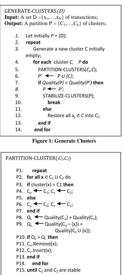
The general schema of the TPC algorithm is specified in Fig. 1. The algorithm starts with a partition having a single cluster i.e whole data set (line 1). The central part of the algorithm is the body of the loop between lines 2 and 15. Within the loop, an effort is made to generate a new cluster by 1) choosing a candidate node to split (line 4), 2) splitting the candidate cluster into two sub-clusters (line 5), and (line 3) calculating whether the splitting allows a new partition with better high degree than the original partition (lines 6–13). If this is true, the loop can be stopped (line 10), and the partition is updated by replacing the original cluster with the new sub-clusters (line 8). Otherwise, the sub-sub-clusters are discarded, and a new cluster is taken for splitting.
The generation of a new cluster calls STABILIZE-CLUSTERS in line 9, improves the overall high degree by trying relocations among the clusters. Clusters at line 4 are taken in increasing order of high degree.
3.1 SPLITTING A CLUSTER
A splitting procedure gives a major improvement in the high degree of the partition. Choose the attribute that gives the highest improvement in the high degree of the partition.
3.2. PARTITION-CLUSTER
Lines P8 and P9 compute the involvement of x to the local high degree in two cases: either x remains in its original cluster (Cu) or x is moved to the other cluster (Cv). If moving x gives an improvement in the local high degree, then the swapping is done (lines P10–P13). Lines P2–P14 in the algorithm is nested into a main loop: elements are continuously checked for swapping until a convergence is met. The splitting process can be sensitive to the order upon which elements are considered: In the first stage, it could be not convenient to reassign the generic xi from C1 to C2, whereas a convenience in performing the swap can be found after the relocation of some other element xj. The main loop partly smoothes this effect by repeatedly relocating objects until convergence is met. Better PARTITION-CLUSTER can be made strongly insensitive to the order with which cluster elements are considered.
Figure 1: Generate Clusters
Figure 2: Partition Cluster
The idea is to rank and sort the cluster elements before line P1, which is on the basis of their splitting effectiveness. To this purpose, each transaction x belonging to cluster C can be associated with a weight w(x), which indicates its splitting effectiveness. x is eligible for splitting C if its items allow us to divide C into two homogeneous sub-clusters. In this respect, the Gini index is a natural way to quantify the splitting effectiveness G(a) of the individual attribute value
a x. Precisely, G(a) = 1 – Pr(a|C)2 – (1 - Pr(a|C))2, where Pr(a|C) denotes the probability of a within C. G(a) is close to its maximum whenever a is present in about half of the transactions of C and reaches its minimum whenever a is unfrequent or common within C. The overall splitting effectiveness of x can be defined by averaging the splitting
effectiveness of its constituting items w(x) = avg a x (G(a)).
Once ranked, the elements x C can be considered in descending order of their splitting effectiveness at line P2. This guarantees that C2 is initialized with elements, which do not represent outliers and still are likely to be removed from C1. This removes the dependency on the initial input order of the data. With decision tree learning, TPC exhibits a preference bias, which is encoded within the notion of homogeneity and can be viewed as the preference for compact clustering trees. Indeed, due to the splitting effectiveness heuristic, homogeneity is enforced by the effects of the Gini index. At each split, this tends to isolate clusters of transactions with mostly frequent attribute values, from which the compactness of the overall clustering tree follows.
3.3 STABILIZE-CLUSTERS
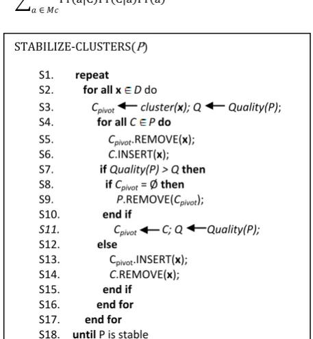
PARTITION-CLUSTER improves the local high degree of a cluster. And STABILIZE-CLUSTERS try to increase partition high degree. It is carried out by finding the most suitable clusters for each element among the ones which are there in the partition.
Fig. 3 shows the pseudo code of the procedure. The central part of the algorithm is a main loop which (lines S2–S17) examines all the available elements. For each element x, a pivot cluster is identified, which is the cluster containing x. Then, the available clusters are continuously evaluated. The insertion of x in the current cluster is done (lines S5–S6), and the updated high degree is compared with the original high degree.
If an improvement is obtained, then the swap is accepted (line S11). The new pivot cluster is the one now containing x, and if the removal of x makes the old pivot cluster empty, then the old pivot cluster is removed from the partition P. If there is no improvement in high degree, x is restored into its pivot cluster, and a new cluster is examined. The main loop is iterated until a stability condition for clusters is achieved.
3.4 Cluster and Partition Qualities
AT-DC gives two different high degree measures, 1) local homogeneity within a cluster and 2) global homogeneity of the partition. As shown in Fig. 1, it is noticed that partition high degree is used for checking whether the insertion of a new cluster is really suitable: it is for maintaining compactness. Cluster high degree in procedure PARTITIONCLUSTER is done for good separation.
Cluster high degree is known when there is a high degree of intracluster homogeneity and intercluster homogeneity. There is strong relation between intracluster homogeneity and the probability Pr(ai|Ck) that item ai appears in a transaction
GENERATE-CLUSTERS(D)
Input: A set D ={x1,…,xN} of transactions; Output: A partition P = {C1,…,Ck} of clusters;
1. Let initially P = {D};
2. repeat
3. Generate a new cluster C initially empty;
4. for each cluster Ci P do 5. PARTITION-CLUSTERS(Ci,C); 6. P’ P U {C};
7. if Quality(P) < Quality(P’) then
8. P P’;
9. STABILIZE-CLUSTERS(P); 10. break
11. else
12. Restore all xj C into Ci; 13. end if
14. end for
15. until no further cluster C can be generated
PARTITION-CLUSTER(C1,C2)
P1. repeat
P2. for all x C1 U C2 do P3. if cluster(x) = C1 then P4. Cu C1; Cv C2; P5. else
P6. Cu C2; Cv C1; P7. end if
P8. Qi Quality(Cu) + Quality(Cv); P9. Qs Quality(Cu – {x}) +
Quality(Cv U {x}); P10.if Qs > Qi then
P11. Cu.Remove(x); P12.Cv.Insert(x); P13.end if P14. end for
containing in Ck. There is a strong relationship between intercluster separation and Pr(x
∈
Ck, ai∈
x). Cluster homogeneity and separation is computed by relating it to the unity of items within the transactions that it contains. Cluster high degree is equal to the combination of the above probability,Pr a|C Pr C|a Pr a
𝑎 ∈ 𝑀𝑐
Figure 3: Stabilize Clusters
The last term is used for weighting the importance of item a in the summation: Essentially, high values from low-frequency items are less relevant than those from high-frequency values. By the Bayes theorem, the above formula is expressed as
Pr(C) Pr a|C 2 𝑎∈𝑀𝑐
Terms Pr (a|C)2 (relative strength of a within C) and Pr(C) (relative strength of C) work in contraposition. It is easy to compute the gain in strength for each item with respect to the whole data set, that is
High deg. (Ck) = Pr(Ck) Pr(a|Ck)2− Pr a|D 2
𝑎 ∈𝑀𝑐𝑘
………. (1) Where,
Ck – cluster
Pr(Ck) – relative strength of Ck a Є MCk – an item
M = {a1,……., am} is set of Boolean attributes Pr(a| Ck) - relative strength of a within Ck Pr(a|D) - relative strength of a within D
D = {x1,…., xn} is data set of tuples defined on M
High degree (Ck) =𝑛𝑁 𝑎 ∈ 𝑥,𝑥 ∈𝐶 𝑛𝑎𝑁 2− 𝑁𝑎𝑁 2 …..…… (2)
Where na and Na represent the frequencies of a in C and D, respectively. The value of High degree (Ck) is updated as soon as a new transaction is added to C.
4.
RESULTS AND ANALYSIS
Two real-life data sets were evaluated. A description of each data set employed for testing is provided next, together with an evaluation of the TPC performances.
Educational Dataset: It contains 50 instances, each having 12 attributes (student name, 9 Boolean attributes and 2 numeric’s). The "type" attribute appears to be the class attribute. In total there are 7 classes of students, that is, class 1 (BE) has 14 set of students, class 2 (BA) has 5 set of students, class 3 (BSc) has 5 set of students, class 4 (BCom) has 6 set of students, class 5 (BCA) has 4 set of animals, class 6 (Polytechnic) has 7 set of animals and class 7 (MBBS) has 9 set of animals. In this dataset, missing Attribute Values is denoted by "?". Table 1 shows that in cluster 1, a class 1, 2 and 5 are having high homogeneity and in cluster 2, classes 4, 6 and 7 are having high homogeneity but it consists of 2 misclassified records in class 3. From figure 4 it can be seen that inter homogenous quality and intra homogeneous quality of clusters 1, 2, 4, 5, 6 and 7 is 100% whereas inter homogenous quality and intra homogeneous quality of cluster 3 is only 30%.
Table 1: Confusion matrix for Educational data
Cluster No. Classes
1 2 3 4 5 6 7
1 12 5 2 0 4 0 0
2 0 0 5 6 0 7 9
Figure 4: Qualities of Clusters
5.
CONCLUDING REMARK
This innovative TPC algorithm is parameter-free, fully-automatic approach to cluster high-dimensional categorical data. The main advantage of our approach is its capability of avoiding explicit prejudices, expectations, and presumptions on the problem at hand, thus allowing the data itself to speak. This is useful with the problem at hand, where the data is described by several relevant attributes.
A limitation of our proposed approach it cannot deal with outliers. Outliers are one that appears to deviate markedly from other members of the sample in which it occurs. Hence, a significant improvement of TPC can be obtained by defining an outlier detection procedure that is capable of detecting and removing outlier transactions before partitioning the clusters.
0%
20%
40%
60%
80%
100%
1
2
3
4
5
6
7
Qu
al
ity
of C
lus
ter
Cluster Number
STABILIZE-CLUSTERS(P)
S1. repeat S2. for all x D do
S3. Cpivot cluster(x); Q Quality(P); S4. for all C P do
S5. Cpivot.REMOVE(x); S6. C.INSERT(x); S7. if Quality(P) > Q then S8. if Cpivot= Ø then S9. P.REMOVE(Cpivot); S10. end if
S11. Cpivot C; Q Quality(P); S12. else
S13. Cpivot.INSERT(x); S14. C.REMOVE(x); S15. end if
S16. end for S17. end for
The research work can be extended further to improve the high degree of clusters by removing outliers.
6.
REFERENCES
[1] J. Grabmeier and A. Rudolph, “Techniques of Cluster Algorithms in Data Mining,” Data Mining and Knowledge Discovery, vol. 6, no. 4, pp. 303-360, 2002.
[2] A. Jain and R. Dubes, Algorithms for Clustering Data. Prentice Hall, 1988.
[3] R. Ng and J. Han, “CLARANS: A Method for Clustering Objects for Spatial Data Mining,” IEEE Trans. Knowledge and Data Eng., vol. 14, no. 5, pp. 1003-1016, Sept./Oct. 2002.
[4] A.M. Bagiwa, S.I. Dishing, “A Conceptual Framework for Extending Distance Measure Algorithm For Data Clustering”, International Journal of Computer Trends and Technology- March to April issue.
[5] G. Gan and J. Wu, “Subspace Clustering for High Dimensional Categorical Data,” SIGKDD Explorations, vol. 6, no. 2, pp. 87-94, 2004.
[6] Y. Yang, X. Guan, and J. You, “CLOPE: A Fast and Effective Clustering Algorithm for Transactional Data,” Proc. Eighth ACM Conf. Knowledge Discovery and Data Mining (KDD ’02), pp. 682-687, 2002.
[7] Eugenio Cesario, Giuseppe Manco, and Riccardo Ortale, “Top-Down Parameter-Free Clustering of High-Dimensional Categorical Data”. IEEE TRANSACTIONS ON KNOWLEDGE AND DATA ENGINEERING, VOL. 19, NO. 12, DECEMBER 2007.
[8] E. Han, G. Karypis, V. Kumar, and B. Mobasher, “Clustering in a High Dimensional Space Using Hypergraph Models,” Proc. ACM SIGMOD Workshops Research Issues on Data Mining and Knowledge Discovery (DMKD ’97), 1997.
[9] M. Ozdal and C. Aykanat, “Hypergraph Models and Algorithms for Data-Pattern-Based Clustering,” Data Mining and Knowledge Discovery, vol. 9, pp. 29-57, 2004.
[10]K. Wang, C. Xu, and B. Liu, “Clustering Transactions Using Large Items,” Proc. Eighth Int’l Conf. Information and Knowledge Management (CIKM ’99), pp. 483-490, 1999.
[11]P. Andritsos, P. Tsaparas, R. Miller, and K. Sevcik, “LIMBO: Scalable Clustering of Categorical Data,” Proc. Ninth Int’l Conf. Extending Database Technology (EDBT ’04), pp. 123-146, 2004.
[12]I. Cadez, P. Smyth, and H. Mannila, “Probabilistic Modeling of Transaction Data with Applications to Profiling, Visualization, and Prediction,” Proc. Seventh ACM SIGKDD Int’l Conf. Knowledge Discovery and Data Mining (KDD ’01), pp. 37-46, 2001.
[13]M. Carreira-Perpinan and S. Renals, “Practical Identifiability of Finite Mixture of Multivariate Distributions,” Neural Computation, vol. 12, no. 1, pp. 141-152, 2000.
[14]G. McLachlan and D. Peel, Finite Mixture Models. John Wiley & Sons, 2000.
[15]C. Fraley and A. Raftery, “How Many Clusters? Which Clustering Method? The Answer via Model-Based Cluster Analysis,” The Computer J., vol. 41, no. 8, 1998.
[16]P. Smyth, “Model Selection for Probabilistic Clustering Using Cross-Validated Likelihood,” Statistics and Computing, vol. 10, no. 1, pp. 63-72, 2000.
[17]D. Pelleg and A. Moore, “X-Means: Extending K-Means with Efficient Estimation of the Number of Clusters,” Proc. 17th Int’l Conf. Machine Learning (ICML ’00), pp. 727-734, 2000.
[18]M. Sultan et al., “Binary Tree-Structured Vector Quantization Approach to Clustering and Visualizing Microarray Data,” Bioinformatics, vol. 18, 2002.
[19]S. Guha, R. Rastogi, and K. Shim, “ROCK: A Robust Clustering Algorithm for Categorical Attributes,” Information Systems, vol. 25, no. 5, pp. 345-366, 2001.
[20]J. Basak and R. Krishnapuram, “Interpretable Hierarchical Clustering by Constructing an Unsupervised Decision Tree,” IEEE Trans. Knowledge and Data Eng., vol. 17, no. 1, Jan. 2005.
[21]Yi-Dong Shen, Zhi-Yong Shen and Shi-Ming Zhang,“Cluster Cores – based Clustering for High – Dimensional Data”.