Edge Responsive Local Directional Patterns
Versus Intensity Dependent Local Patterns:
Implementation and Comparative Analysis
Renu S. Patil Vijay B. Baru
PG Student Associate Professor Department of Electronics & Telecommunication
Engineering
Department of Electronics & Telecommunication Engineering
Sinhgad College of Engineering, Vadgaon (Bk), Pune, India Sinhgad College of Engineering, Vadgaon (Bk), Pune, India
Abstract
Local Patterns are an effective way to construct the descriptors of features where local characteristics are considered to be of importance. Such patterns find their use in the task of face recognition and more importantly expression recognition. This paper focuses on the implementation of the intensity variant patterns and the directional pattern for the purpose of expression recognition. The performance of the feature descriptors is compared for the performance analysis. This comparison is carried out on the basis of the recognition time and the recognition efficiency obtained. The system uses both the types of feature extractors one by one and forms the feature vectors from them. These feature vectors are then used to classify the expressions present in the image. The classifier used for the implementation of system is Support Vector Machine. The aim of this paper is to implement the intensity variant local patterns and the edge responsive directional patterns and compare them on the basis of their performance for expression recognition. The conclusion drawn from the comparison is that the edge responsive patterns are more suitable for the feature description than the intensity variant patterns. The patterns that are considered for implementation are Local Binary Pattern and Local Directional Number Pattern. For a broader analysis, the higher order variants such as Ternary and Derivative Pattern are also implemented.
Keywords: Local Patterns, Feature Descriptors, Feature Vectors, Expression Recognition, Local Binary Pattern, Local Directional Number Pattern
________________________________________________________________________________________________________
I. INTRODUCTION
Features play an important role in the description of an object, a face and pretty much anything. Accurate description of features is vital for the purpose of successful implementation of computer vision. A generic block diagram for a recognition system suitable for computer vision implementation is given below.
Fig. 1: Block Diagram for Generic Approach to Computer Vision
The data in this case is generally two-dimensional, wherein the system deals with image and video. The step of data acquisition is carried out with the help of various pre-processing techniques, such as color image to gray level conversion, edge detection by making use of various filtering techniques or illumination and occlusion correction. The step of data representation is done by the various feature extractors and descriptors that have been developed with time. For Object detection, the prevalent techniques that are used are Scale-Invariant Feature Transform (SIFT) [1], Speeded-Up Robust Features (SURF)[2], Oriented FAST and Rotated BRIEF (ORB) [3]. These feature descriptors are global. Contrary to the object detection, the face and expression recognition requires local operation for the detection and extraction of features. The descriptors that can be used for the task of face recognition, expression recognition and texture recognition. These descriptors are Local Binary Pattern [4] and its higher order variants and the newly developing edge responsive patterns the prominent example of which is the Local Directional Number Pattern [5].
II. FEATURE DESCRIPTORS FOR IMPLEMENTATION
This section gives an introduction of the Local Feature descriptors that are implemented for the comparative analysis. They can be classified into two, namely, Intensity variant local patterns and edge responsive local directional patterns. The detailed description is given in the following sub-sections.
Intensity variant Local Patterns
The most prominent intensity variant local patterns is the Local Binary Pattern introduced by Ojala et al [4]. This operator makes use of the neighborhood intensities to form a binary code which can be used to describe the pixel of interest and form a feature vector which can be used further for classification. The description of Local Binary Pattern can be given in the following way.
Consider a monochrome image I (x, y) and let gc denote the gray level of an arbitrary pixel (x, y), i.e. gc=I(x, y). Moreover, let gp denote the gray value of a sampling point in an evenly spaced circular neighborhood of P sampling points and radius R around point (x,y):
gp = I (xp, yp), p = 0, . . . , P – 1 (1) xp = x +R cos(2πp/P) (2) yp = y −R sin(2πp/P) (3) Where,
gp= gray value of sampling point in the circular neighborhood, gc= gray level value of pixel of interest
xp= x co-ordinate of the radius of circular region yp= y co-ordinate of the radius of circular region
Assuming that the local texture of the image I (x, y) is characterized by the joint distribution of gray values of P +1 (P > 0)
pixels:
T = t (gc,g0,g1, . . . , gP−1)
Without loss of information, the center pixel value can be subtracted from the neighborhood: T = t (gc,g0 −gc,g1 − gc, . . . , gP−1 −gc)
In the next step the joint distribution is approximated by assuming the center pixel to be statistically independent of the differences, which allows for factorization of the distribution:
T ≈ t (gc)t (g0 −gc,g1 − gc, . . . , gP−1 −gc)
(4) Reliable estimation of this multidimensional distribution from image data can be difficult.
The learning vector quantization based approach has certain unfortunate properties that make its use difficult. First, the differences gp − gc are invariant to changes of the mean gray value of the image but not to other changes in gray levels. Second, in order to use it for texture classification the codebook must be trained similar to the other texton-based methods. In order to alleviate these challenges, only the signs of the differences are considered:
t (s(g0 − gc), s(g1 − gc), . . . , s(gP−1 − gc)) Where s(z) is the thresholding (step) function.
s(z) = {0, z < 0
1, z ≥ 0 (5)
The generic local binary pattern operator is derived from this joint distribution. As in the case of basic LBP, it is obtained by summing the threshold differences weighted by powers of two. The LBPP,R operator is defined as
LBPP,R(xc, yc) = ∑ s(gp− gc)2p p−1
p=0 (6)
The above equation means that the signs of the differences in a neighborhood are interpreted as a P -bit binary number, resulting in 2P distinct values for the LBP code. The local gray-scale distribution, i.e. texture, can thus be approximately described with a 2P -bin discrete distribution of LBP codes:
T ≈ t (LBPP, R(xc ,yc)) (7)
The LBP code is calculated for each pixel in the cropped portion of the image, and the distribution of the codes is used as a feature vector, denoted by S:
S = t (LBPP, R(x,y)) (8) Where,
t(LBP)= Joint distribution of the codes
In practice, the LBP equation signifies that the sign of the differences that are obtained by comparing the center pixel and the pixels surrounding are seen as a P -bit binary number, that result in 2Pseparate values for the LBP code. Uniform LBP patterns are used for better facial recognition as they are more stable and fewer samples are required for their reliable estimation of distribution. Also, use of uniform LBP patterns helps in dealing with the dimensionality problem, i.e. the 256 bin histograms are reduced to 59 bins only due to the uniform patterns that are considered.
𝑠𝑡𝑒𝑝(𝑖, 𝑖𝑐, 𝑡) = {
1, 𝑖 ≥ 𝑖𝑐+ 𝑡
0, |𝑖 − 𝑖𝑐| < 𝑡
−1, 𝑖 ≤ 𝑖𝑐− 𝑡
(9)
In which, i is the interest pixel, icis the pixel at the center and t is the value of the threshold that is decided on the amount of changes that are to be allowed in the pixel values without affecting the thresholding results. An example of a Local Ternary operator is given as follows. In the following example, the obtained LTP code is converted into two LBP codes in order to take care of the dimensionality reduction. These two LBP codes are subsequently called as upper LBP pattern and lower LBP pattern. Same as LTP there exists a Quaternary code wherein the values are split into five (-2,-1,0,1,-2). These can be split into four LBP patterns. The Local Derivative Pattern operator was proposed for face recognition and the focused areas were feasibility of the high-order local patterns and their effectiveness for representation of face [10]. In this approach, LBP, in concept, is regarded as the non-directional first-order operator, all-directional first-order derivative result is encoded by LBP and the higher-order derivative information which consists of detailed discriminative features is encoded by LDP. This information is such that the first-order pattern cannot be used for obtaining it from an image.
Edge Responsive Directional Patterns
Edge responsive Directional Patterns are derived from the sharpening filters that are used for the extraction of the information. The pattern is called as Local Directional Number Pattern. LDN encodes the structure of a local neighborhood by analyzing its directional information. Consequently, we compute the edge responses in the neighborhood, in eight different directions with a compass mask. Then, from all the directions, we choose the top positive and negative directions to produce a meaningful descriptor for different textures with similar structural patterns. This approach allows us to distinguish intensity changes (e.g., from bright to dark and vice versa) in the texture, that otherwise will be missed. In order for the LDN code to be obtained, the first step is to compute the entire image with the Kirsch compass masks. There are eight such masks and they are given as follows.
M0= [
−3 −3 5
−3 0 5
−3 −3 5
]; M1= [
−3 5 5
−3 0 5
−3 −3 −3
]; M2= [
5 5 5
−3 0 −3
−3 −3 −3
]; M3= [
5 5 −3
5 0 −3
−3 −3 −3
];
M4= [
5 −3 −3
5 0 −3
5 −3 −3
]; M5= [
−3 −3 −3
5 0 −3
5 5 −3
]; M6= [
−3 −3 −3
−3 0 −3
5 5 5
]; M7= [
−3 −3 −3
−3 0 5
−3 5 5
]
These masks are applied to the image and the LDN code is obtained by analyzing the edge response of each mask, {M0,…,M7} that represents the edge significance in its respective direction, and by combining the dominant directional numbers. Given that the edge responses are not equally important; the presence of a high negative or positive value signals a prominent dark or bright area. Hence, to encode these prominent regions, we implicitly use the sign information, as we assign a fixed position for the top positive directional number, as the three most significant bits in the code, and the three least significant bits are the top negative directional number.
Therefore, we define the code as:
LDN(i, j) = 8xi,j+ yi,j (10)
Where (i,j) is pixel in the center of the neighborhood that is converted into a code, xi,j is the maximum positive response directional number of the, and yi,j is minimum negative response directional number that are defined as follows.
xi,j= arg max {∏ (i, j)|0 ≤ x ≤ 7}xx (11)
yi,j= arg max {∏ (i, j)|0 ≤ y ≤ 7}yy (12)
The gradient space is used instead of the intensity feature space, to compute the code. The former has more information than the later, as it holds the relations among pixels implicitly (while the intensity space ignores these relations). Moreover, due to these relations the gradient space reveals the underlying structure of the image.
III. EXPERIMENTS
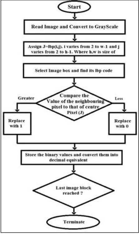
The algorithms that are implemented are given in the form of the flowcharts. These flowcharts are followed by a brief description about how the algorithms are applied to the available dataset.
Intensity variant Operators
pixel is greater, the neighboring pixel value is replaced with a ‘0’ else it is replaced with ‘1’. The binary string of such ones and zeros forms the LBP code for that pixel of interest. All such pattern codes are calculated in turn and the LBP code for the entire image can be obtained. The approach towards LTP is very much similar to LBP. However, in order to deal with the susceptibility of LBP to the noise introduced in the monotonic gray level changes, a threshold ‘t’ is used. This threshold can be assigned arbitrarily and with trial and error metho d. The advantage of this alteration is that instead of a single value comparison between the neighboring pixel and the center pixel, a range of values is available which minimizes the impact of noise. The separation of the matrix into upper and lower binar y pattern is carried out as demonstrated in the earlier chapter, i. e. replacing -1 by 0 for upper binary pattern and replacing 1 by 0 for lower binary pattern. Thus, in place of one, the output is two histograms. The concatenation of both these histograms per block leads to the formulation of the feature vector. The Local Derivative Pattern encodes the directional information of the four directions namely 0°, 45°, 90° and 135°. The codes that are obtained along these directions can be displayed in the form of images as shown below. The histograms of these images are converted into feature vectors by the means of concatenation. The length of the feature vector increases by four fold than Local Binary Pattern.
Fig. 2: Flowchart of Local Binary Pattern
Edge Responsive Directional Patterns
The edge responsive local directional number pattern is implemented as per the following algorithm. 1) Read the image.
2) Divide the image into small regions
3) Apply the seven kirsch masks to each region and obtain the dominant directional information. 4) By using the sign information, obtain the top negative and top positive directional numbers.
5) Combine these such that the first three most significant digits are positive directional numbers and the last three least significant digits are negative directional numbers.
6) Represent the region by an LDN histogram
The image is converted to grayscale for the application of the kirsch masks. An alternative is the Derivative-Gaussian mask, which can be varied in size as per the requirement. After the application of the kirsch masks, the directional information is extracted for the formation of the histogram for feature vectors. The advantage of using the gradient information is that it provides a robustness towards noise and illumination changes.
IV. RESULTS
The algorithms that are mentioned in the previous section are applied to the two databases for the comparison of their performance. The results are predominantly for the Local Binary Pattern and Local Directional Number Pattern. Both these algorithms are applied for the feature extraction from the images from the JAFFE database as well as the self-created database. The results after applying the feature extractors are given in this section.
LBP Operator Results
The following figures give a demonstration of the intensity variant patterns applied to datasets.
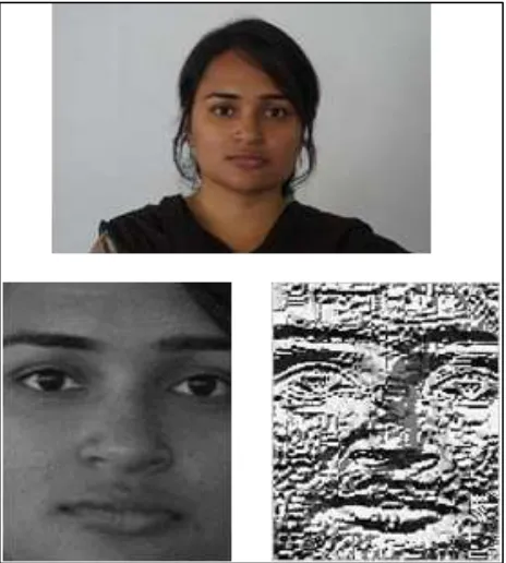
Fig. 3(a): Original Image from JAFFE database. (b): LBP coded image
Along with the JAFFE database, the LBP is also applied to the self-created database. The results are given in the following figure.
Fig. 4(a): Original image, (b): ROI extracted grayscale image and (c): LBP coded image
LDN Operator Results
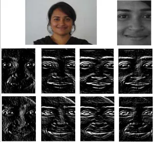
Fig. 5(a): Original Image from JAFFE database (b): M0 masked image (c): M1 masked image (d): M2 masked image (e): M3 masked image (f): M4 masked image (f): M5 masked image (g): M6 masked image (h): M7 masked image
As in the case of JAFFE database images, the directional operator is also applied for the self-created database. The figure below indicates the original color image from the database, the gray scale image that is obtained for the purpose of ease of application of operator and the images obtained after Kirsch masking.
The following table gives the idea of the performance of the algorithms that are considered in this paper. The performance is judged against time that is required for processing. The parameters are training time required for the JAFFE dataset without region of interest (ROI) extraction, training time required for JAFFE dataset with ROI extraction, training time required for self-created dataset without ROI extraction, training time required for self-self-created dataset with ROI extraction, recognition time required without ROI for JAFFE images, recognition time with ROI for JAFFE images, recognition time without ROI for self-images, recognition time with ROI for self-images. The mentioned parameters are very important for commenting about the efficiency of the intensity as well as the directional information extraction for the purpose of machine vision.
Table – 1
Algorithms and their timing performance
Parameters Algorithms
LBP LTP LDP LDN
Number of Feature Vectors 59 128 1024 56
Training time of full JAFFE image (sec) 25.7016 33.408 45.054 34.1619 Training time with ROI extraction in JAFFE image (sec) 23.748 14.8023 20.8307 12.1347 Recognition time without ROI extraction (sec) 2.79 4.04 7.31 1.23
Recognition time with ROI extraction (sec) 1.84 3.53 6.8 0.98 Training time for self-created images (sec) 11.6529 14.8987 5.5084 10.6704 Recognition time for self-created images (sec) 1.12 2.65 3.87 0.74
V. CONCLUSION
Local Binary Pattern is a good intensity variant feature descriptor. The performance it offers rivals the directional operators. However, the loss of information is a major factor because of which the directional patterns are considered to be of vitality. The Local Directional Number Pattern that is implemented in this paper has 56 feature vectors, 3 less than the least computationally complex local binary pattern, which has 59. These 59 vectors are computed by obtaining by combining the similar uniform patterns into 56 types and the rest non-uniform patterns into 3 feature vectors. The time that is taken for training and recognition by LDN is less than LBP and much better than LTP or LDP as seen from the table. Moreover, the variants, though they extract more information than their parent operator, fail to provide the timing efficiency that is given by the edge responsive directional pattern.
ACKNOWLEDGEMENT
A sincere gratitude towards the Head of Department, Dr. M.B. Mali, department of Electronics and Telecommunication SCOE, and Dr. S. D. Lokhande, Principal, SCOE, Pune for their encouragement for this paper
REFERENCES
[1] S. Keypoints and D. G. Lowe, “Distinctive Image Features from Scale-Invariant Keypoints,” Comput. Vis., vol. 60, no. 2, pp. 91–110, 2004.
[2] H. Bay, T. Tuytelaars, and L. Van Gool, “Surf: Speeded up robust features,” Lect. notes Comput. Sci., vol. 3951, p. 14, 2006.
[3] E. Rublee and G. Bradski, “ORB : an efficient alternative to SIFT or SURF.”
[4] T. Ojala, M. Pietikäinen, and T. Mäenpää, “Multiresolution Gray Scale and Rotation Invariant Texture Classification with Local Binary Patterns,” pp. 1–35.
[5] A. R. Rivera, S. Member, J. R. Castillo, and S. Member, “Local Directional Number Pattern for Face Analysis : Face and Expression Recognition,” no. c,
pp. 1–13, 2011.
[6] M. Learning, M. Learning, K. A. Publishers, K. A. Publishers, A. C. Sciences, A. C. Sciences, R. August, and R. August, “Induction of Decision Trees,”
Expert Syst., pp. 81–106, 2007.
[7] A. Technologies and S. Dutta, “AN APPROACH TO RECOGNIZE FACIAL EXPRESSIONS USING LOCAL,” no. 3, pp. 60–64, 2014.
[8] S. A. Nazeer, N. Omar, and M. Khalid, “Face Recognition System using Artificial Neural Networks Approach,” pp. 420–425, 2007.
[9] X. Tan and B. Triggs, “Enhanced Local Texture Feature Sets for Face Recognition Under Difficult Lighting Conditions,” pp. 168–182, 2007.