ISSN (e): 2250-3021, ISSN (p): 2278-8719 Vol. 04, Issue 05 (May. 2014), ||V1|| PP 07-17
Vibration Analysis Of Beam Subjected To Moving Loads Using
Finite Element Method
Arshad Mehmood
1, Ahmad Ali Khan
2, Husain Mehdi
3 1(Mechanical Engineering, Zakir Husain College of Engineering & Technology/AMU/INDIA) 2
(Mechanical Engineering, Zakir Husain College of Engineering & Technology/AMU/INDIA) 3
(Meerut Institute Technology /UPTU/INDIA)
Abstract: - It was purposed to understand the dynamic response of beam which are subjected to moving point loads. The finite element method and numerical time integration method (Newmark method) are employed in the vibration analysis. The effect of the speed of the moving load on the dynamic magnification factor which is defined as the ratio of the maximum dynamic displacement at the corresponding node in the time history to the static displacement when the load is at the mid – point of the structure is investigated. The effect of the spring stiffness attached to the frame at the conjunction points of beam and columns are also evaluated. Computer codes written in Matlab are developed to calculate the dynamic responses. Dynamic responses of the engineering structures and critical load velocities can be found with high accuracy by using the finite element method
Keywords: - Beam, Finite Element methods, Numerical tine Integration method ,Dynamic magnification factors, Stiffnes, Shape Function. Critical load Velocity
I. INTRODUCTION
Vibration analysis of structures has been of general interest to the scientific and engineering communities for many years. These structures have multitude of applications in almost every industry. The aircraft industry has shown much interest in this, some of the early solutions were motivated by this industry. This study deals with the finite element analysis of the monotonic behaviour of beams, slabs and beam-column joint sub assemblages. It is assumed that the behaviour of these members can be described by a plane stress field. Reinforced concrete has become one of the most important building materials and is widely used in many types of engineering structures. The economy, the efficiency, the strength and the stiffness of reinforced concrete make it an attractive material for a wide range of structural applications. For its use as structural material, concrete must satisfy the following conditions:
(1) The structure must be strong and safe. The proper application of the fundamental principles of analysis, the laws of equilibrium and the consideration of the mechanical Properties of the component materials should result in a sufficient margin of safety against collapse under accidental overloads.
(2) The structure must be stiff and appear unblemished. Care must be taken to control deflections under service loads and to limit the crack width to an acceptable level.
[5]Wang & Lin (1998) studied the vibration of multi-span Timoshenko frames due to moving loads by using the modal analysis. [6]Kadivar & Mohebpour (1998) analyzed the dynamic responses of unsymmetrical composite laminated orthotropic beams under the action of moving loads. [7]Hong & Kim (1999)presented the modal analysis of multi span Timoshenko beams connected or supported by resilient joints with damping. The results are compared with FEM.[8] Ichikawa et al. (2000) investigated the dynamic behaviour of the multi-span Continuous beam traversed by a moving mass at a constant velocity, in which it is assumed that each span of the continuous beam obeys uniform Euler-Bernoulli beam Theory.
II. DYNAMIC ANALYSIS BY NUMERICAL INTEGRATION
Dynamic response of structures under moving loads is an important problem in engineering and studied by many researchers. The numerical solution can be calculated by various methods which are as follows
1. Duhamel Integral
2. Newmark Integration method 3. Central difference Method 4. Houbolt Method
5. Wilson ϴ Method
III. NEWMARK FAMILY OF METHODS
The New mark integration method is based on the assumption that the Acceleration varies linearly between two instants of time. In 1959 Newmark presented a family of single-step integration methods for the solution of structural Dynamic problems for both blast and seismic loading. During the past 45 years Newmark method has been applied to the dynamic analysis of many practical engineering structures. In addition, it has been modified and improved by many other researchers. In order to illustrate the use of this family of numerical integration methods, we considered the solution of the linear dynamic equilibrium equations written in the following form:
[M]u t +[C]u t+[K]ut= Ft (1)
Where M is the mass matrix, C is the damping matrix and K is the stiffness matrix.
u, u , and u are the acceleration, velocity and displacement vectors, respectively.Ft is the external loading vector. The direct use of Taylor’s series provides a rigorous approach to obtain the following two additional equations:
ut = ut −∆t + ∆tu t −∆t + ∆t2
2 u t −∆t+ ∆t3
6 ut −∆t+……….. (2)
u t = u t −∆t + ∆tu t −∆t+ ∆t2
2 ut −∆t+………... (3)
New mark truncated these equations and expressed them in the following form:
ut = ut −∆t + ∆tu t −∆t + ∆t2
2 u t −∆t+ β∆t
3u+……….
(4)
u t = u t −∆t + ∆tu t −∆t+γ∆t2u+………. (5)
If the acceleration is assumed to be linear within the time step, the following equation can be written as
u = u t−u t −∆t
∆t (6)
The substitution of equation (6) into Equations (4) and (5) produces new mark’s equations in standard form
ut=ut −∆t+∆tu t −∆t+( 1 2−β)∆t
2u
t −∆t+β∆t2u t+……….. (7) u t=u t −∆t+ (1-γ)∆tu t −∆t+γ∆tut+……….. (8)
Stability of Newmark Method
For zero damping Newmark method is conditionally stable if γ≥1
2 , β≤ 1
2 and ∆t ≤ 1
ωmax (γ2−β)
(9)
Whereωmaxis the maximum frequency in the structural systemNew mark’s method is unconditionally stable if
2≥ 1
2 (10)
However, if is greater than 1/2, errors are introduced. These errors are associated with “numerical damping”
and “period elongation”. For large multi degree of freedom structural systems the time step limit, given by
equation (9), can be written in a more usable form as
∆t Tmin≤
1
2π (γ
2−β)
(11)
Where Tmin is the minimum time period of the structure. Computer model of larger structures normally contain
select a numerical integration method that is unconditionally stable for all time steps. Table 3.1 shows the summary of the Newmark method for direct integration.
IV. SOLUTION USING FINITE ELEMENT METHOD
Finite element method (FEM) is a numerical method for solving a differential or integral equation. It has been applied to a number of physical problems, where the governing differential equations are available. The method essentially consists of assuming the piecewise continuous function for the solution and obtaining the parameters of the functions in a manner that reduces the error in the solution.
A promising approach for developing a solution for structural vibration problems is provided by an advanced numerical discretisation scheme, such as, finite element method (FEM).The finite element method (FEM) is the dominant discretisation technique in structural mechanics.
The basic concept in the physical FEM is the subdivision of the mathematical model into disjoint (non-overlapping) components of simple geometry called finite elements or elements for short. The response of each element is expressed in terms of a finite number of degrees of freedom characterized as the value of an unknown function, or functions, at a set of nodal points. The response of the mathematical model is then considered to be approximated by that of the discrete model obtained by connecting or assembling the collection of all elements. The finite element method (FEM) is the dominant discretisation technique in structural mechanics. The basic concept in the physical interpretation of the FEM is the subdivision of the mathematical model into disjoint (non-overlapping) components of simple geometry called finite elements or elements for short. The response of each element is expressed in terms of a finite number of degrees of freedom characterized as the value of an unknown function, or functions, at a set of nodal points.
The response of the mathematical model is then considered to be approximated by that of the discrete model obtained by connecting or assembling the collection of all elements. The disconnection-assembly concept occurs naturally when examining many artificial and natural systems. For example, it is easy to visualize an engine, bridge, building, airplane, or skeleton as fabricated from simpler components. Unlike finite difference models, finite elements do not overlap in space.
V. BEAM ELEMENT
Beams are the most common type of structural component, particularly in Civil and Mechanical Engineering. A beam is a bar-like structural member whose primary function is to support transverse loading and carry it to the supports. The main difference of beams with respect to bars is the increased order of continuity required for the assumed transverse-displacement functions to be admissible. Not only must these functions be continuous but they must possess continuous x first derivatives. To meet this requirement both deflections and slopes are matched at nodal points. Slopes may be viewed as rotational degrees of freedom in the small-displacement assumptions used here.
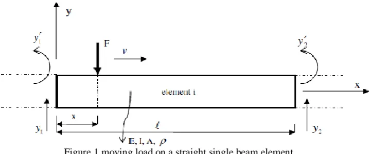
A beam is another simple but commonly used structural component. It is also geometrically a straight bar of an arbitrary cross-section, but it deforms only in directions perpendicular to its axis. A straight beam element with uniform cross section is shown in Figure1.The main difference between the beam and the truss is the type of load they carry. Beams are subjected to transverse loading, including transverse forces and moments that result in transverse deformation. Finite element equations for beams will be developed for the analysis, and the element developed is known as the beam element.
Figure 1 moving load on a straight single beam element
divided into shorter beams, where each can be treated as beam(s) with a uniform cross-section. Nevertheless, the Finite element matrices for varying cross-sectional area can also be developed with ease using the same concepts that are introduced. The beam element developed is based on the Euler–Bernoulli beam theory that is applicable for thin beams.
The Euler-Bernoulli beam theory is used for constituting the finite element matrices. The longitudinal axis of the element lies along the x axis. The element has a constant moment of inertia I, modulus of elasticity E, density ρ and length l. Two degrees of freedom per node, translation along y-axis (y1, y2) and rotation about z-axis ( y1’,
y2’) are considered. The beam is modeled with 20 equally sized elements.
VI. ANALYSIS OF BEAM ELEMENT
Consider a beam element of length l= 2a with nodes 1 and 2 at each end of the element, the local x-axis is taken in the axial direction of the element with its origin at the middle section of the beam. Similar to all other structures, to develop the FEM equations, shape functions for the interpolation of the variables from the nodal variables would first have to be developed. As there are four DOFs for a beam element, there should be four shape functions. It is often more convenient if the shape functions are derived from a special set of local coordinates, which is commonly known as the natural coordinate system. This natural coordinate system has its origin at the centre of the element, and the element is defined from −1 to +1, as shown in Figure2.
Figure2 beam element having 2 nodes with 4 dofs
Finite Element Method Equation
In planar beam elements there are two degrees of freedom (DOFs) at a node in its local coordinate system. They are deflection in the y direction, and rotation in the x–y plane, with respect to the z-axis. Therefore, each beam element has a total of four DOFs.
The beam is divided into elements having each nodes has two degree of freedom. Typically the degree of freedom of node1 are q1 and q2 , and for node2 are q3 and q4.the vector represents the global displacement vector
for a single element the local degree of freedom are represented by:
q = q1,q2,q3,q4 T
(11) since q is same as y1,y 1,y 2,y2
T
.The shape function for interpolating y on an element are defined in terms of on -1 to +1 since nodal values and nodal shapes are involved .we define hermit shape functions which satisfy nodal value and slope continuity requirement’s each of the shape functions is of cubic order represented by H = a + b + c2 + d3 (12) Where a, b, c and d are four unknown constants which are determined by imposing the boundary conditions at the corresponding nodes.
The following conditions must be satisfied as:
values H1 H1 H2 H2 H3 H3 H4 H4
= -1 1 0 0 1 0 0 0 0
= 1 0 0 0 0 1 0 0 1
The coefficients a, b, c and d are easily obtained by imposing these conditions in equation (12) obtained as: H1 =
1
4 2 − 3 + 3
(13) H2 =
1
4 1 − −
2+ 3
(14)
H3 =
1
4 2 + 3 −
3
(15) H4 =
1
4 −1 −+ 2
The hermits shape function can be used to write function y () in the form y() = H1y1 + H2
dy
d 1 + H3y2 +H4
dy
d (17)
x= 1−
2 x1 + 1+
2 x2 (18)
=x1+x2
2 + x2−x1
2 (19)
Since the length of the element l= x2-x1
We have dx =l
2d
(20) y0 = H1q1 +
l
2H2q2 + H3q2 + l
2H4q4
(21)
y=Hq (22) Where H= H1,l
2H2,H3, l
2H4 (23)
We consider the integral as summations over the integrals over the elements. The element strain energy of a single element is given by
S.E= EI
2 l 0 (
∂2y ∂x2)
2dx (24)
dy dx=
2 l
dy d and
d2y d x2 =
4 l2
d2y
d2x (25)
Then substituting y=H q we obtain
d2y dx2
2
= qT16
l4
d2H d2
T d2H
d2 q (26)
d2H
d2 =
3 2,
−1+3 2
l 2, −
3 2,
1+3 2
l
2 (27)
S.E = 12qT 8EI l3
9 4
2 3
8(−1 + 3)l − 9 4
2 3
8(1 + 3)l −1+3
4 2
l2 −3
8(−1 + 3)l
−1+92
16 l 2
symmetric 9
4
2 −3
8(1 + 3)l 1+3
4 2
l2 +1
−1 dξq (28)
This result the elemental strain energy is given by
S.E=1/2 qTK q (29)
the symmetric elemental stiffness matrix becomes as
K= EI
l3
12 6l −12 6l 6l 4l2
−6l 2l2
−12 6l −6l 2l2 12 −6l −6l 4l2 (30)
Similarly Using M= +1HT −1 HρA
l
2d (31)
On integration we get
M = 420ρAl
156 22l 54 −13l 22l 4l2 13l −3l2
54 −13l 13l −3l2 156 −22l −22l 4l2 (32)
The overall mass and stiffness matrices of the structure M and K are constituted by joining 20 element matrices using Mat lab codes,
Equations of Motion of the Beam Structure
The equation of motion for a multiple degree of freedom undamped structural system is represented as follows
[M]{y } + [K] {y} = {F (t)} (33)
Where y and y are the respective acceleration and displacement vectors for the whole structure and F (t) is the external force vector.
[[K] − ω2
[M]] {Φ} =0 (34)
Where ω is the angular natural frequency and Φ is the mode shape of the structure for the corresponding natural frequency.
Beam specification:
Software used Mat lab codes
Parameter Frequency
Length of beam 1m
Section dimensions 0.01×0.01m2
Boundary conditions a) Clamped –clamped b) Clamped-pinned c) Pinned-pinned
Material Steel
Mass density 7860 kgm‐3 Elastic modulus 206.0E09Nm‐2 Two different spring stiffness K1=50000N/m
K2=200000N/m
The dynamic analysis is performed for beam and frame geometry and obtained the natural frequencies of the structure. Beams which are under considerations are subjected to constant point force F = -100 N is used. The moving point load on a beam having three different boundary conditions gives us different frequencies. The first three natural frequencies of the beam element are obtained for Using Mat lab given in table1
Table1 the first three natural frequency of the beam Natural frequency(HZ)
Modes 1 2 3 BEAM
Clamped-clamped 52.62 145.06 284.39 Clamped-pinned 36.26 117.52 245.21 Pinned-pinned 23.21 92.86 208.93
VII. CONCLUSION
Analytical Solution of Beam under Moving Load with different boundary condition using Dynamic Green Function
The governing equation of a flexible beam subject to a concentrated moving force, shown in Fig. 5.1, can be given by
4 2
4 2
( , )
( , )
( , )
y x t
y x t
EI
F x t
x
t
(38)Fig. 3, Moving mass on a beam with general boundary condition
3 2
3 2
( , )
( , )
( , )
( , )
l t
y x t
y x t
y x t
k y x t
k
x
x
x
for x=0 and x=l (39)( , 0)
( , 0)
y x
0
y x
t
(40)where
k
l andk
t are linear and twisting spring constants, that prevent vertical motion and in x-y plane rotation of the beam ends, respectively.F x t
( , )
is external load and for a moving concentrated load case, can be given byF x t
( , )
P
(
x u
)
(41) WhereP
is the amplitude of the applied load, and
is the Dirac-delta function, which is defined by0 0
(
x
x
) ( )
f x dx
f x
(
)
(42)Results of the Dynamic Analysis of Beam
Fig4 Matlab results for clamped – clamped boundary conditions of a beam with values
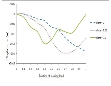
Fig5 Dynamic displacements of the mid – point of the clamped – clamped beam versus the position of the moving load on the beam for various α values
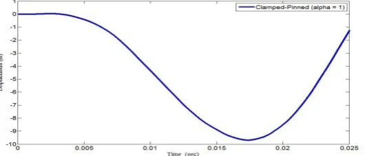
Fig 7 Dynamic displacements of the mid – point of the clamped – pinned beam versus the position of the Moving load on the beam for various α values
Fig8 Matlab results for pinned – pinned boundary conditions of a beam witvalues
Figu10 dynamic magnification factor of the mid - point of the beam versus α for three different boundary conditions.
Figure 4 shows the dynamic responses of the mid-points of the clamped – clamped beam for value before discussing about the numerical results the formulation developed herein is validated against available analytical solutions for a beam with different boundary conditions and acted upon by a moving load. First, comparison of the analytical results with the matlab results of a clamped-clamped beam as given in table 5.1
The vertical axis in Fig. 5, shows the dimensionless deflections (
y
y y
/
st) of the point under the moving load, and the horizontal axis depicts the position of the load along the beam. Results reported by are computed by assumed mode method and are compared with the present result of green function approach. As it can be observed in Fig. 6, there is an excellent agreement between the two results. Wherey
st is the static transverse deflection at the beam mid span when a concentrated load with amplitude F is applied statically at the beam's mid span. For example for the clamped – clamped B.C. we have:yst=
Fl3
192EI
(43)
In Fig. 7, deflection of a beam with simply supported boundary conditions for the speed parameter α=2 dimensionless speed parameter defined as:
cr
v
v
(44)Where the critical speed is:
m
EI
l
T
l
v
cr
2
(45)
Where
EI
is the bending rigidity,m
is the mass per unit length of the beam and T is the period that is related to lowest mode of beam vibrations. In Fig. 8, there is a close agreement between the analytical result and that obtained by matlab codesThe speed parameter as mentioned is ratio of speed of the load to critical speed. In this article, the speed parameter is introduced in the following form
αi=
v
ωil ; i=1,2,3….
(46)
Where
v
is the speed of load inm
s
and
i is thei
t hnatural frequency of beam inrad
s
. Fig 4, 5, 6 show the mid – point displacements versus the position of the moving load on the beam for different boundary0.9 1 1.1 1.2 1.3 1.4 1.5 1.6 1.7 1.8
0 0.2 0.4 0.6 0.8 1 1.2 1.4 1.6 1.8 2
Dy
n
am
ic
M
agn
if
ic
at
io
n
F
ac
to
r
α
conditions and various values for the beam structure. With small values (=0.01) displacement curve is close to the static displacement curve for all boundary conditions(clamped-clamped, clamped-pinned, pinned-pinned). The moving load and the maximum dynamic displacements of the mid-point of the beam are not in the same phase at overcritical part. The time at which the maximum mid – point displacement is observed shifts right with increasing values regardless of the boundary condition of the beam. The highest dynamic deflections occur for the pinned – pinned beam as expected.
Fig 10 shows the dynamic magnification factor (Dd) of the mid - point of the beam versus for three
different boundary conditions. The maximum dynamic magnification occurs for = 1.02 and Dd = 1.632 for
clamped – clamped beam. For the clamped – pinned beam the maximum value of the dynamic magnification is 1.662 and observed at = 1.31. For pinned – pinned beam, the maximum Dd= 1.728 and recorded at =
1.22. For pinned – pinned boundary conditions the dynamic magnification values are greater than those obtained for clamped –clamped and clamped – pinned beams for low and high moving load speeds. The clamped – clamped boundary conditions generally gives the lower dynamic magnification values except in the middle speed region.
Dynamic magnification factors for the mid – point of the beams are given for various values and different boundary conditions in Table 2. These values are only valid in the time interval that the moving load is on the beam.
Table2 Dynamic magnification factors for the mid – point of the beams for various a values (*α values which makes Dd maximum)
VIII. CONCLUSION
Moving load problem is generally studied for beam structures. In addition to the beam structures, dynamic responses of frames and spring attached frames subjected to the moving point load are also analyzed in this study. Euler-Bernoulli beam theory is used in the finite element method for constituting the element matrices. The Newmark integration method is employed for forced vibration analysis. The conclusions drawn can be summarized as follows:
1. The moving load and the maximum dynamic displacements for the mid-point of the beam are not in the same phase at overcritical part. The time at which the maximum mid – point displacement is observed shifts right with increasing α values regardless of the boundary condition of the beam.
2. The highest dynamic displacements occur for a pinned – pinned beam. For pinned – pinned boundary conditions the dynamic magnification values are greater than those obtained for clamped – clamped and clamped – pinned beams for low and high moving load speeds. The clamped – clamped boundary conditions generally gives the lower dynamic magnification values except the middle speed region.
3. Attaching a spring to the frame at the conjunction points of beam and columns makes the frame more rigid and shifts the mode shapes of the frame structure up.
4. A longer beam implies a smaller first natural frequency for frame structure ;similarly longer columns imply smaller natural frequencies.
5. With lower α values (α <1 ) springs are very effective for all nodes. In this interval, higher Dd values are
obtained with increasing spring stiffness. In the middle and high speed region, attaching a spring to the frame is not an advisable solution due to the increasing Dd values.
6. Maximum Dd occurs after the moving load left the beam for both columns and beam of the frame structure
when the α value is greater than some critical values.
7. Lower Dd values are observed with increasing damping ratio for a clamped –clamped beam. The occurring
time of maximum dynamic displacement shifts left with increasing damping ratio.
REFERENCES
[1] Bilello, C. & Bergman, L.A. (2004) Vibration of damaged beams under a moving mass: theory and experimental validation. Journal of Sound and Vibration, 274, 567-582.
[2] Biggs J. M. (1982) Introduction to Structural Dynamics McGraw-Hill, New York Chen, Y.H., Huang, Y.H. & Shih, C.T. (2001) Response of an infinite Timoshenko beam on a viscoelastic foundation to a harmonic moving load. Journal of Sound and Vibration 241(5) 809-824.
[3] Chopra, Anil K. (1995) Dynamics of Structures, Prentice Hall, New Jersey. Clough R.W., Penzien, J. (1993) Dynamics of Structures. New York: McGraw-Hill.
[4] Hanselman, Duane C. (2001) Mastering Matlab 6. Prentice Hall, Upper Saddle River, N.J.
[5] Hong, S.W. & Kim, J.W. (1999) Modal analyses of multi span Timoshenko beams connected or supported by resilient joints with damping. Journal of Sound and Vibration, 227(4), 787-806.
[6] Ichikawa, M., Miyakawa, Y. & Matsuda, A. (2000) Vibration analysis of the continuous beam subjected to a moving mass. Journal of Sound and Vibration, 230(3), 493-506.
[7] Kadivar, M.H. & Mohebpour, S.R. (1998) Finite element dynamic analysis of unsymmetric composite laminated beams with shear effect and rotary inertia under the action of moving loads. Finite Elements in Analysis and Design (29) 259-273
[8] Wu, J.J., Whittaker, A.R. & Cartmell, M.P. (2001) Dynamic responses of structures to moving bodies using combined finite element and analytical methods. International Journal of Mechanical Sciences (43) 2555-2579
[9] Zibdeh, H.S. & Hilal, M.A. (2003) Stochastic vibration of laminated composite coated beam traversed by a random moving load. Engineering Structures (25) 397-404
[10] Wu, J.J., Whittaker, A.R. & Cartmell, M.P. (2001) Dynamic responses of structures to moving bodies using combined finite element and analytical methods. International Journal of Mechanical Sciences (43) 2555-2579
[11] Rao, Singiresu S. (1995) Mechanical Vibrations. Addison - Wesley Publishing Company.
[12] Chandrupatla.R.Tirupathi and Belegundu.D Ashok Introduction to finite elements in Engineering, third edition
[13] Oniszczuk, Z. (2003) Forced transverse vibrations of an elastically connected complex simply supported double-beam system. Journal of Sound and Vibration, 264, 273-286