Face Mole Detection, Classification and Application
Chen-Chiung Hsieh
*, Jun-An Lai
Department of Computer Science and Engineering, Tatung University, No. 40, Sec. 3, JhongShan N. Rd., Taipei, Taiwan.
* Corresponding author. Tel.: 886-21822928 Ext. 6571; email: [email protected] Manuscript submitted September 14, 2013; accepted August 15, 2014.
doi: 10.17706/jcp.10.1.12-23
Abstract: Do you have moles on face? Are the moles good or bad? We could treat this problem from medical, cosmetic, or even fortune applications viewpoint. Here, image processing techniques are investigated to detect and verify the goodness of face mole from fortune telling point of view. The process includes Voronoi diagram setup for sample moles, face mole detection, and mole recognition. In the first part, Voronoi diagram is used to partition the given sample mole-face into regions. In the second part, face detection and Laplacian of Gaussian is used to get the prominent features on face. Aspect ratio and area are two features for mole verification. At last, an algorithm is developed to warp the detected user moles to the sample mole-face by Thin-plate Spline Analysis for mole recognition. By using Voronoi diagram, the mole recognition spends only O(logn), where n is the number of given sample moles. The goodness of the recognized mole could be retrieved according to the stored information for fortune telling. The system was tested with 20 people and the mole recognition rate reached 91.25% which demonstrated the feasibility of the proposed system.
Key words: Active shape model, face analysis, pattern recognition, Voronoi diagram.
1.
Introduction
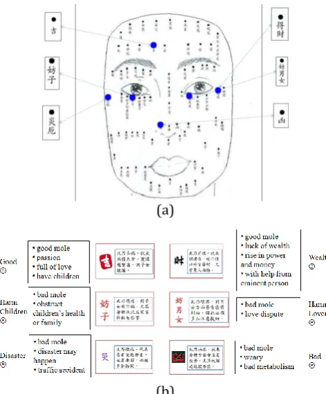
Moles on face puzzle people and people seek ways like laser care to remove the acne like spots. However, some moles look beautiful and good from viewpoint of fortune telling, people may tend to keep the moles. Contrarily, some moles are bad for fortune telling and people would tend to eliminate these annoying spots on face. In this paper, we proposed an automatic mole classification system based on the given fortune telling sample-mole [1] as shown in Fig. 1(a). Therefore, people could make a judgment whether to keep their moles or not based on the classification results.
Traditionally, mole fortune telling is conducted by meeting a fortune teller face to face. However, there are several disadvantages of traditional fortune telling. Some fortune tellers may make use of fortune telling to defraud people. In addition, it is also hard to search for a good fortune teller. Fig. 1(b) shows an APP for fortune telling. However, there is only a sample face with reference moles on face just like Fig. 1(a). There is no automatic mole recognition process and customized friendly user interface for mole based fortune telling currently.
organized as follows. Section 2 gives some related researches in mole recognition. Section 3 presents the detail of our method which is divided into three parts. The first part is to partition sample mole-face into Voronoi diagram for user mole classification. The second part is to detect face by Haar-like features and extract facial components by ASM. This is to do mole extraction with facial components not considered. Laplacian of Gaussian filter is adopted to find mole candidates. In the last part, warp detected user moles to the sample mole-face for mole recognition by the mole Voronoi diagram generated in the first part. Thin plate spline analysis (TPS) is adopted to do face warp and the detected mole could be classified as the given mole within the same Voronoi cell. User specific fortune information could then be retrieved from database according to the recognized moles. Section 4 describes the experimental results. Finally, we make conclusions in the last section.
(a) (b)
Fig. 1. (a) The given fortune telling sample moles [1] are represented by black dots and named in Chinese. (b) An App in apple store for mole reading from:
http://itunes.apple.com/us/app/molereading-zhi-ban-ming- xiang/id420210170?mt=8.
2.
Related Works
Usually, mole detection is used to increase face recognition rate or to predict tumor. Lee et al. [2] proposed a detection method of moles on human back torso with recognition rate 90%. Mean shift [3] is used to locate mole candidates and noises are removed by morphological operations. Aspect ratio and shape are then used to filter out false positives. Pierrard et al. [4] proposed a face mole detection method using normalized cross correlation (NCC) [5] and 3D morph model that are more resistant to lighting and face gesture. However, only prominent moles are found and the recognition rate is 87%. Cho et al. [6] detected moles by firstly applying skin color detection on input image. Difference of Gaussian (DoG) filter is then used to find candidate moles on detected skin regions. Steerable filter [7] and a graphical model [8] are also applied to remove noises like hairs. Support Vector Machine (SVM) [9] is finally adopted to recognize the moles. The recognition rate is 79% due to the effects caused by hairs on skin.
for face detection and facial components extraction need to be adaptive for each individual. In addition, detected face needs to be warped to the sample mole-face for adaptive recognition capability. These problems are solved and discussed in the following sections.
3.
System Architecture
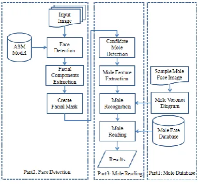
Fig. 2 depicted the proposed system architecture. The first part is utilizing Voronoi diagram to partition the sample mole-face for positioning the detected moles. The second part is face detection by Haar-like features and facial component extraction by Active Shape Model (ASM). An adaptive facial mask is generated in which facial components are excluded. For the last part, mole detection is conducted by DoG filter on the masked face and filtered again by the properties of area and shape (aspect ratio). These detected moles are warped by Thin-plate Spline Analysis (TPS) to the sample mole-face and are recognized as the nearest defined moles in the calculated Voronoi diagram. Finally, related fortune information could be retrieved from database according to the recognized moles.
Fig. 2. System architecture.
3.1.
Mole Voronoi Diagram
The moles on one’s face usually are not exactly at the same positions as those given sample moles. To classify the detected moles on one’s face, one of the better ways is by the nearest-neighbour classifier. Therefore, Voronoi diagram [10], [11] is used to partition the given sample mole-face into cells in which each defined sample mole is located at the center of the cell. Each detected mole dm is then classified as the defined mole m if dm falls within the region belonging to m.
(a) (b)
Voronoi diagram is a tool for geometric applications. Given a set of site points P = {P1, P2, …, Pn}, on a 2D
plane, it is to partition the space into regions according to (1) in which Euclidean distance is adopted. Each point x is in the region of Pi if Pix is less than all the other distances Pjx,ji. The partitioned region for Pi is called the Voronoi cell of Pi. The set of all the Voronoi cells as in (2) is called the Voronoi diagram
V(P). An example is given in Fig. 3(a). Points that are of equal distances to the neighboring sites are on the edges called Voronoi edge and the intersection points are called Voronoi vertex. To partition the sample mole-face as shown in Fig. 1(a) into cells for each defined mole, an algorithm of O(nlogn) is applied to find the mole Voronoi diagram as shown in Fig. 3(b).
xP x P x j i
P
V( i) i j , (1)
( ), ( ),..., ( )
)( V P1 V P2 V Pn
V P (2)
3.2.
Face Detection
To achieve the goal of mole classification, the system needs to detect face and extract facial components with respect to different people. Then, mole detection and positioning could be processed on detected face. To build a deformable shape model for variety of human faces, ASM [12] was utilized to detect and extract facial components. The main advantage is that different target could be detected by training the corresponding samples. ASM is described briefly in the following.
3.2.1.
Active shape model
Positive samples are used to train ASM. In our system, there are 75 landmarks including feature points of face shape, eyebrow, eyes, nose, and mouth as shown in Fig. 4. These feature points are selected manually because they are of corner points, high curvature, or junction points. Interpolated points are inserted at equal distance between two consecutive feature points. A set of landmarks for a face is represented by x as in (3), where n is the number of landmarks.
x T
n n y
x y x y
x, , , ,..., , )
( 1 1 2 2
(3)
Fig. 4. Selected landmark points in the proposed system.
where
x
j and yj are as in (5)-(6) and M is the number of training data. T n n y x y x yx, , , ,..., , )
( 1 1 2 2
x (4)
M i ij j n
x M 1 ,..., 2 , 1 , 1 j
x (5)
M
i i
j j n
y M 1 ,..., 2 , 1 , 1 j
y (6)
From all the training data and mean shape, a covariance matrix S of 2n×2n could be calculated by (7). By singular value decomposition of the covariance matrix, Eigen-system consists of Eigenvalue λ(λ1, λ2,…, λ2n)
and Eigenvector P(P1, P2, …, P2n) was obtained. There are 2n feature values in the feature space. We could
choose only the most important t features as in (8).
M i T i i M 1 ) )( ( 1 x x x xS (7)
98 . 0 , 2 1
1
f f n i i t i i
(8)ASM was built by the mean shape and Eigen-system as in (9) after all the above training processes were completed.
b
x
x
P
, (9) where b is a variable representing the feature vector. ASM varies according to the changes in b as in (10), where m=2~3. We could verify the range of ASM scope b from a set of known shape xas in (11), where P must be of square matrix to insure the existence of transpose matrix of P.i i
i b m
m
(10)
)
(
x
x
b
P
T
(11) Before the first change, b is set as zero to get the target shape which is equal to the mean shape. Then, the shape of ASM could be changed by varying b. Furthermore, shape and position parameters could be adjusted to change the rotation angle and scaling factor for a deformable ASM as in (12) and (13), where s is the scaling factor, is the rotation angle, and (Tx, Ty) is the translational offset.
) ( )
( x Pb
xA p (12)
y x T T s s s s p A cos sin sin cos )
( (13)
3.2.2.
Facial mask
In our Color independent face detection proposed by Viola and Jones [13] and extended by Lienhart and Maydt [14] is adopted. The characteristic of this method is the use of the black-white haar-like patterns to detect whether the current considered region containing two eyes. Though this method is independent to the skin color of people, false alarms would happen at eyes-like spots. In this paper, false alarms would be filtered out if the number of skin pixels within the detected face region is less than a given threshold [15].
An example is given as shown in Fig. 5. All the defined 75 feature points could be extracted from the detected face as shown in Fig. 5(a). Those extracted facial feature points are used to generate a facial mask as shown in Fig. 5(b) for mole detection. I.e., the black area will be ignored in the following steps.
(a) (b)
Fig. 5. ASM on a detected face. (a) Extracted feature points by ASM. (b) Generated facial mask.
(a) (b)
(c) (d)
Fig. 6. (a) Gaussian smoothing filter [15]. (b) Gaussian smoothing operator. (c) Laplacian operator. (d) Laplacian of Gaussian filter [16].
3.3.
Mole Detection and Classification
Mole detection, face warping, and mole recognition are described in this section.
3.3.1.
Mole detection
(a) (b) (c) (d)
Laplacian of Gaussian [16] integrates Gaussian smoothing filter [17] and Laplacian operator [18] to detect points which vary dramatically from surroundings. Since it is a high pass filter and therefore Gaussian smoothing filter is often used to filter noises. In Fig. 6(a), the effect of smoothing is controlled by adjusting . The larger , the more smooth result.
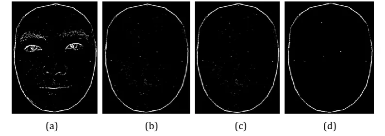
Laplacian filter operator as shown in Fig. 6(c) is a second order derivative operator as defined in (14). It is combined with Gaussian filter as in (15) to form the so called Laplacian of Gaussian and the corresponding high pass filter is shown as in Fig. 6(d). Fig. 5(a) after Laplacian of Gaussian filter is given in Fig. 7(a). The prominent facial features including facial components, facial shape, moles, and scars are all detected. By applying the facial mask as shown in Fig. 5(b), the resulting image is as shown in Fig. 7(b). In order to extract the moles accurately, morphological closing is conducted to fill holes and then connected component could be used to extract the moles as shown in Fig. 7(c).
2 2 2 2 ) , ( ) , ( ) , ( y y x f x y x f y x L
(14)
2 2 2 2 2 2 2 4 2 1 1 ) , ( y x e y x y x LoG
(15)
The extracted connected components are only mole candidates and need to be verified by height/width ratio and area size. The height/width aspect ratio as in (16) is used to filter out those parts that are of thin shape like hair and the area size as in (17) is to filter out small noises. The final detected moles on Fig. 5(a) are as shown in Fig. 7(d).
8 . 1 5
.
0
width height
Mole
Mole (16)
2
5 . 1 pixel
MoleArea (17)
3.3.2.
Face warping
To position the recognized moles on the sample mole-face, we need to warp user face to the sample mole-face. Not only feature points of user face shape are mapped to the feature points of referenced sample face, but also feature points of the facial components need to be mapped to those feature points of sample mole-face.
We adopted Thin-plate Spline Analysis (TPS) [19] to map all the 75 feature points to the sample mole-face. The most important work is to map the detected moles to the sample mole-face by the same transformation equation. The theoretical foundation is to treat the user face image as a thin plate which is deformed by external force. Find the corresponding points of those original feature points by using the deformed thin plate for new coordinate calculation. According to TPS, we can deduce the mapping matrix by using equations of force and energy. Firstly, give two sets of feature points denoted by Pi (xi,yi) and
) , ( i i i X Y
h , where Pi and hi are the control points of plane A and B, respectively. We could obtain a
transformation equation Φ defined in (18) to map all points in plane A to plane B.
n i i i yxx a y U P P
a a P
1
1 ( )
)
( , (18)
where P(x, y) is any point in plane A and
P
P
i is the Euclidean distance between P and any control point Pi. We could get the corresponding coordinate in plane B by substituting P(x, y) in (18). 0 0 0 2 1 2 21 1 12 n n n n U U U U U U
K , (19)
where Uij rij2logrij and rij PiPj is the distance between control points.
n n y y y x x x Q 2 1 2 1 1 1 1
, (20)
where (xi,yi),i1,2,...,n, is the control point in plane A. Then matrix L of size (n3)(n3)could be calculated from K and Q as in (21).
0 T Q Q K
Q , (21)
Finally, the coefficients
1
n,a
x anda
y in (18) could be calculated by (22).T L a a a
W n x y T
1 1
1 )
(
, (22)
where
Tn
h h h
T 1 2 0 0 0 and hi (xi,yi),i1,2,...,n, is the control points in plane B.
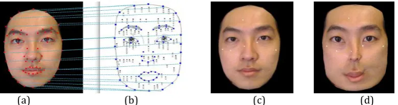
The set of ASM feature points on detected user face is set P on A and the set of ASM landmark points on the standard mole sample face is set h on B. TPS modeling is to calculate the necessary coefficients for warping the landmark points P to h. Then, the new coordinates for detected user mole points could be warped to sample mole-face for fating process. Fig. 8 gives an example of TPS warping from a detected user face in Fig. 8(a) to the sample mole-face in Fig. 8(b). Note the landmark points belonging to the inner region of mouth are ignored. The detected moles in Fig. 8(c) are mapped to the new locations as shown in Fig. 8(d). The warped image looks similar to the sample mole-face proves the mapping is successful. In summary, the mole reading algorithm is then described as follows.
(a) (b) (c) (d)
Fig. 8. Mapping the detected moles to the standard mole-face by TPS. (a) The landmarks on a detected user face. (B) The landmark points on the standard mole-face. (c) Detected moles on a user face. (b) Warped face
after TPS mapping.
Algorithm: Mole recognition
Input: Voronoi diagram of the sample mole-face and the detected user (mole) face.
Output: Retrieved fate information for each recognized mole.
Step 1. [TPS Modelling] Apply TPS to warp the ASM landmark points from detected user face to the sample mole-face.
Step 2. [Mole Warping] Warp the detected moles to the standard mole-face by the TPS model computed in Step 1.
1http://www.opencv.org.cn/index.php/Download
detected moles. The Voronoi diagram computed previously thus could be deployed to solve this problem. According to the coordinates of warped moles in Step 2, an O(logn) algorithm could be used to decide which Voronoi cell contains the warped mole, where n is the number of given sample moles. Note the boundary of NNDR is the Voronoi edge between Voronoi cells. There are other solutions. To analyse the time complexity, the one-by-one comparison to get the nearest sample mole is O(n). However, the mole recognition spends only O(log n) by using Voronoi diagram.
Step 4. [Information retrieval] According to the found Voronoi cells, retrieve corresponding fate information from mole fate database.
(a)
(b)
Fig. 9. (a) The recognized moles are indicated with bigger dots for the user in Fig. 5. (b) The retrieved fate information corresponding to the recognized moles shown in (a) originally in Chinese are translated to
English.
Fig. 9 shows the result after mole recognition for the user in Fig. 8. The corresponding fate information for each recognized mole is retrieved as shown in the textbox in Fig. 9. Both Chinese and English versions are given. As the accuracy of the fate information is up to the user and for user reference only. Here we pick the original explanation from [1] without any inference. In which, good mole is represented by a smiling face and bad mole by a sad face.
4.
Experimental Results
Our system was developed using Visual Studio 2008 on Windows XP Professional. The proposed mole reading system is intended to be used in real time. The face detection module is modified from OpenCV1
example code located in the sample directory of OpenCV distribution. The hardware platform is a PC with Intel®Core™2 Q6600 CPU @2.4GHz and 2GB main memory. The camera adopted is Logitech web camera C905 and image resolution is set as 640×480.
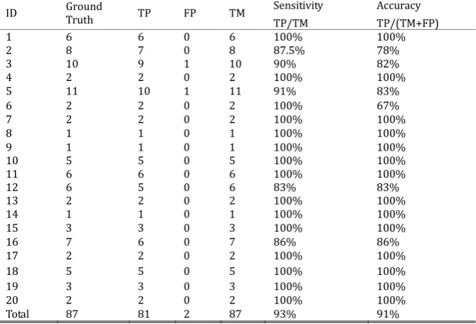
these 20 images is 87 in total. The recognized moles were marked by larger dots in the last column. To measure the system performance, (23) and (24) are adopted to calculate the sensitivity and diagnostic accuracy.
TM TP y
Sensitivit (23)
FP TM
TP Accuracy
Diagnostic
, (24)
In which, TP represents True Positive, the number of moles in images and are detected, and FP, False Positive, is the number of false moles which are detected as moles. TM represents the number of total moles in images. From experimental results as shown in Table 2, the Sensitivity is 93.65% and the Diagnostic Accuracy is 91.25%. Some of the errors were caused by hair, eyebrow, moustache, acne, or scars as shown in Fig. 10. In addition, moles on edges of facial components may not be detected.
Table 1. Partial Test Subjects and the Recognized Moles
Original Image Detected Moles Warped Image Mole Positioning
Table 2. Accuracy for Mole Detection
ID Ground Truth TP FP TM Sensitivity Accuracy
TP/TM TP/(TM+FP)
1 6 6 0 6 100% 100%
2 8 7 0 8 87.5% 78%
3 10 9 1 10 90% 82%
4 2 2 0 2 100% 100%
5 11 10 1 11 91% 83%
6 2 2 0 2 100% 67%
7 2 2 0 2 100% 100%
8 1 1 0 1 100% 100%
9 1 1 0 1 100% 100%
10 5 5 0 5 100% 100%
11 6 6 0 6 100% 100%
12 6 5 0 6 83% 83%
13 2 2 0 2 100% 100%
14 1 1 0 1 100% 100%
15 3 3 0 3 100% 100%
16 7 6 0 7 86% 86%
17 2 2 0 2 100% 100%
18 5 5 0 5 100% 100%
19 3 3 0 3 100% 100%
20 2 2 0 2 100% 100%
Total 87 81 2 87 93% 91%
image per person was taken. The positioning accuracy was 98.6%. Some of the errors were caused by the ASM in which the facial shape was not correctly modeled as shown in Fig. 10(g) and 10(h). However, once the ASM modeling was done correctly, the detected moles could be warped to the sample mole-face and recognized by the Voronoi diagram as one of the sample mole without error.
(a) (b) (c) (d)
(e) (f) (g) (h)
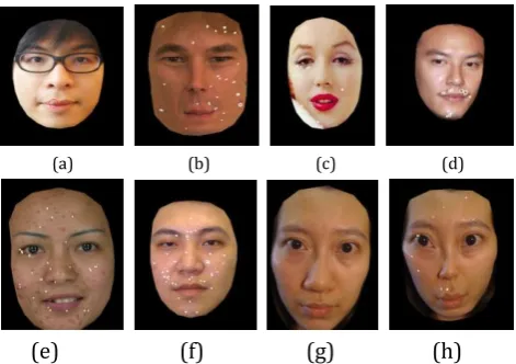
Fig. 10. Errors analysis of proposed mole detection. (a) Mole on edge or lip. (b) Hair effect. (c) Eyebrow effect. (d) Moustache effect. (e) Acne effect. (f) Scar effect. (g) ASM positioning error. (h) TPS warping of (g).
5.
Conclusion
This paper proposed a mole classification system. It is consisted of three parts, the sample mole distribution map for mole recognition, mole detection, and mole recognition process. The sample mole distribution map is firstly constructed by partitioning the standard sample mole-face into Voronoi diagram in which each defined mole locates at the center of its Voronoi cell. Active shape modelling (ASM) could be used to extract facial feature points from the detected face. Laplacian of Gaussian is applied to find the moles on detected face. Aspect ratio and area size are used to filter out the wrong ones. Then the detected moles are warped to the created sample mole Voronoi diagram. The detected mole would be recognized as the defined mole centred at the same Voronoi cell. By that defined sample mole id, we could retrieve the corresponding fate information for that mole. Experimental results showed that the accuracy of mole recognition reached 91.25% which demonstrated the feasibility of proposed system. Do you have moles? What do you think about these moles? This system may give you a hint.
References
[1] Mole reading. (2012, September). From http://55-website.com/xo3/67/6709/168.htm
[2] Lee, T. K., Atkins, M. S., King, M. A., Lau, S., & McLean, D. I. (2005). Counting moles automatically from back images. IEEE Trans. on Biomedical Engineering, 52(11), 1966-1969.
[3] Comaniciu, D., & Meer, P. (2002). Mean shift: a robust approach toward feature space analysis. IEEE
Trans. on Pattern Analysis and Machine Intelligence, 24(5), 603-619.
[4] Pierrard, J. S., & Vetter, T. (2007) Skin detail analysis for face recognition. Proceeding of CVPR (pp. 1-8). [5] Wei, S. D., & Lai, S. H. (2008). Fast template matching based on normalized cross correlation with
adaptive multilevel winner update. IEEE Trans. on Image Processing, 17(11), 2227-2235.
[6] Cho, T. S., Freeman, W. T., & Tsao, H. (2007). A reliable skin mole localization scheme. Proceedings of
the 11th IEEE International Conference on Computer Vision (pp. 1-8).
[7] Freeman, W. T., & Adelson, H. (1991). The design and use of steerable filters. IEEE Trans. on Pattern
[8] Tappen, M. F., Russell, B. C., & Freeman, W. T. (2004). Efficient graphical models for processing images.
Proceedings of the 2004 IEEE Conference on Computer Vision and Pattern Recognition: Vol. 2 (pp.
II-673-II-680).
[9] Cristianini, N., & Taylor, J. S. (2000). An Introduction to Support Vector Machines. Cambridge University Press.
[10]Riviere, S., & Schmitt, D. (2007). Two-dimensional line space Voronoi diagram. Proceedings of the 4th
International Symposium on Voronoi Diagrams in Science and Engineering (pp. 168-175).
[11]Zhao, Y., Liu, S. J., & Zhang, Y. H. (2012). Spatial density Voronoi diagram and construction. Journal of
Computers, 7(8), 2007-2014.
[12]Cootes, T. F., Taylor, C. J., Cooper, D. H., & Graham, J. (1995). Active shape models — Their training and application. Computer Vision and Image Understanding, 38-59.
[13]Viola, P., & Jones, M. (2001). Rapid object detection using a boosted cascade of simple features.
Proceedings of the 2001 IEEE Conference on Computer Vision and Pattern Recognition CVPR: Vol. 1 (pp.
511-518).
[14]Lienhart, R., & Maydt, J. (2002). An extended set of Haar-like features for rapid object detection.
Proceedings of 2002 International Conference on Image Processing: Vol. 1 (pp. 900-903).
[15]Hsieh, C. C., Liou, D. H., & Lee, D. (2010). A robust hand gesture recognition system using Haar-like features. Proceedings of the 2nd International Conference on Signal Processing and Systems (pp. V2-394-V2-398). Dalian, China.
[16]Tabbone, S. (1994). Detecting junctions using properties of the Laplacian of Gaussian detector. Proceedings of the 12th IAPR International Conference on Computer Vision & Image Processing Pattern
Recognition: Vol.1 (pp. 52-56).
[17]Gaussian smoothing. (2014, Oct.). From http://homepages.inf.ed.ac.uk/rbf/HIPR2/gsmooth.htm [18]Laplacian of Gaussian. (2014, Oct.). From http://homepages.inf.ed.ac.uk/rbf/HIPR2/log.htm
[19]Bookstein, F. L. (1989). Principal warps: thin-plate splines and the decomposition of deformations.
IEEE Trans. on Pattern Analysis and Machine Intelligence, 11(6), 567-585.
[20]Kumar, M. P., Torr, P. H. S., & Zisserman, A. (2007). An invariant large margin nearest neighbor classifier. Proceeding of IEEE 11th International Conference on Computer Vision (pp. 1-8).
[21]Gao, Y., Zheng, B., Chen, G., Lee, W. C., Lee, K. C. K., & Li, Q. (2009). Visible reverse k-nearest neighbour query processing in spatial databases. IEEE Trans. on Knowledge and Data Engineering, 21(9), 1314-1327.
Chen-Chiung Hsieh received the B.S., M.S., and Ph.D. degrees all in the Department of Computer Science and Information Engineering, National Chiao-Tung University, Hsinchu, Taiwan, in 1986, 1988, and 1992, respectively. During Dec. 1992 to Jan. 2004, he was with the Institute for Information Industry (III) as a vice director. From Dec. 2004 to Jan. 2006, he joined Acer Inc. as a senior director. He is presently an associate professor in the Department of Computer Science and Engineering at Tatung University, Taipei, Taiwan. His research area is mainly focused in image and multimedia processing.
![Fig. 1. (a) The given fortune telling sample moles [1] are represented by black dots and named in Chinese](https://thumb-us.123doks.com/thumbv2/123dok_us/7813635.1663398/2.595.142.463.238.449/given-fortune-telling-sample-moles-represented-black-chinese.webp)