An Adaptive Cauchy Differential Evolution
Algorithm with Bias Strategy Adaptation
Mechanism for Global Numerical Optimization
Tae Jong Choi and Chang Wook Ahn
Department of Computer Engineering, Sungkyunkwan University (SKKU) 2066 Seobu-ro, Suwon 440-746, Republic of Korea
{gry17, cwan}@skku.edu
Abstract—Appropriately adapting mutation strategies is a challengeable problem of the literature of the Differential Evolution (DE). The Strategy adaptation Mechanism (SaM) can convert a control parameter adaptation algorithm to a strategy adaptation algorithm. To improve the quality of optimization result, the exploration property is important in the early stage of optimization process and the exploitation property is significant in the late stage of optimization process. To ensure these, we modified the SaM for strictly controlling a balance between the exploration and the exploitation properties, which called the bias SaM (bSaM). We extended the Adaptive Cauchy Differential Evolution (ACDE) by attaching the bSaM. We compared the bSaM with SaM and the bSaM extended ACDE with the state-of-the-art DE algorithms in various benchmark problems. The result of the performance evaluation showed that the bSaM and the bSaM extended ACDE performs better than SaM and the state-of-the-art DE algorithms not only unimodal but also multimodal benchmark problems.
Index Terms—Differential Evolution Algorithm, Adaptive Strategy Control, Adaptive Parameter Control, Exploration Property, Exploitation Property
I. INTRODUCTION
The Differential Evolution (DE) which Storn and Price proposed [1] is population based robust and powerful stochastic search algorithm for continuous space. This algorithm attempts to improve individuals (elements of population) iteratively for finding global optimum(s). This algorithm is simple and contains fewer control parameters than other Evolutionary Algorithms. This advantage attracts many researchers and leads to apply it in many practical problems. The general and detailed information about the DE can be found in [2].
There are three main control parameters in the DE. They are Scaling Factor, Crossover Rate, and Population Size. They have an effect on in optimization performance highly. The result of setting difference between appropriate parameter values and unsuitable parameter
values is huge. Although the DE contains few control parameters, the combination of the values of control parameters is infinite. Moreover, there are many mutation strategies which contain different optimization properties. Similar to control parameter case, the result of setting difference between an appropriate mutation strategy and an unsuitable mutation strategy is also huge. Therefore, it is necessary that users should find out the appropriate values of control parameters and mutation strategies in advance. To find out these, users usually utilized the trial-and-error search method. However, this method requires a lot of computational time and space [3-13].
The Strategy adaptation Mechanism (SaM) [8] can convert a control parameter adaptation algorithm to a strategy adaptation algorithm. There are many adaptive parameter control algorithms which show robust and powerful optimization performances. Therefore, by utilizing the SaM, users might easily adapt mutation strategies. The SaM utilizes the strategy probability. The authors of the SaM recommend the SaM with JADE’s [7] adaptive parameter control algorithm for adapting the strategy probability, which performs better than jDE [3] and Uniform distribution adaptive parameter control algorithms.
To improve the quality of optimization result, the exploration property is important in the early stage of optimization process and the exploitation property is significant in the late stage of optimization process [11]. To ensure these properties, we modified the SaM for strictly controlling a balance between the exploration and the exploitation properties, which called the bias SaM (bSaM). We extended the Adaptive Cauchy Differential Evolution (ACDE) [10] by attaching bSaM. The ACDE shows good optimization performance by its adaptive parameter control without adaptive strategy control. We compared the bSaM with SaM and the bSaM extended ACDE with the state-of-the-art DE algorithms in various benchmark problems. The result of the performance evaluation showed that the bSaM is better than the SaM and the ACDE’s adaptive parameter control is better than the JADE’s adaptive parameter control in terms of adapting the strategy probability. In addition, we found out that the Long-tailed distribution still performs better than the Short-tailed distribution for the bSaM.
This work was supported under the framework of international cooperation program managed by National Research Foundation of Korea (NRF-2013K2A1B9066056).
This paper proceeds as follows. In Section 2, we introduce the standard DE and the ACDE. In Section 3, we describe the proposed algorithm. In Section 4, we present and discuss the result of the performance evaluation. In Section 5, we conclude this paper.
II.RELATED WORK
A. DE Algorithm
The DE [1] is population based stochastic search algorithm for continuous space. Population is a set of
NP individuals. An individual is D-dimensional vectors.
D G i G i G
i x x
X ,
1 ,
, = " represents an individual. Initialization
operator initializes population as follows:
) ( ] 1 , 0
[ max min min 0 , j j j j
i x rand x x
x = + ⋅ − . (1)
Here, D
x x
X min
1 min
min= " and
D x x X max 1 max
max = " represent
the minimum and the maximum bounds of the search space of optimization problem.
There are three main operators in the DE. They are Mutation, Crossover, and Selection. The purpose of Mutation and the Crossover operators is that increase the diversity of population. The purpose of Selection operator is that removes some inferior individuals. The following is one of the mutation operators, called DE/rand/1/bin.
) ( 2, 3, ,
1
,G r G r G r G
i X F X X
V = + ⋅ − . (2)
Here, Vi,G represents a mutant vector and Xr1,G, Xr2,G,
and Xr3,G represent some donor vectors. The following is
one of the Crossover operators, called Binomial crossover.
⎩ ⎨ ⎧ = j G i j G i j G i x v u , , , otherwise or [0,1)
ifrand ≤ CR j = jrand . (3)
Here, Ui,G represents a trial vector. The following is
Selection operator. ⎩ ⎨ ⎧ = + G i G i G i X U X , , 1 , otherwise ) (X ) (U
if f i,G ≤ f i,G
. (4)
Here, f(Ui,G) and f(Xi,G) represent the fitness values
of the trial vector and the target vector. The DE executes these operators until it satisfying some termination conditions.
A. ACDE
The authors of the ACDE [10] recommend that applying the Long-tailed distribution to the arithmetic mean of a set of successfully evolved individuals’ control parameters at every generations, which can accelerate optimization performance. The followings are the control parameter adaptation of the ACDE.
) 1 . 0 , ( avg
i C F
F = . (5)
) 1 . 0 , ( avg
i C CR
CR = . (6)
Here, C , Favg , and CRavg represent the Cauchy
distribution, the arithmetic mean of a set of successfully evolved individuals’ Scaling Factors, and the arithmetic mean of a set of successfully evolved individuals’ Crossover Rates. The ACDE adapts control parameters appropriately, which leads to robust and powerful optimization performance.
III. THE PROPOSED ALGORITHM
This section describes the strategy adaptation extended ACDE algorithm in detail. The first subsection discuses the strategy pool. The next subsection discuses the strategy adaptation.
A. Strategy Pool
In the proposed algorithm, we applied two mutation strategies. The followings are the strategies.
1) DE/rand/1/bin
2) DE/current-to-best/3/bin
We applied the first mutation strategy for supporting the exploration properties. It performs slow convergence but it has small risk about getting stuck some local minimums. We applied the second mutation strategy for promoting the exploitation properties. It performs fast convergence but it has high probability about getting stuck some local minimums. To increase the number of perturbation vectors can reduce this probability. Therefore, we applied the second mutation strategy instead of best/1/bin or DE/current-to-best/2/bin.
B. Strategy Adaptation
The SaM can convert a control parameter adaptation algorithm to a strategy adaptation algorithm. K and
} , 2 , 1 { K
SK = " represent the number of mutation
strategies in the strategy pool and the strategy pool. Each individual contains the strategy probability,
) 1 , 0 [
,G∈ i
η .The following is the strategy adaptation of the SaM.
⎣
,⎦
1, = ⋅K +
SiG ηiG . (7)
The value of the strategy probability determines one of mutation strategies in the strategy pool. For example, if
2 =
K and ηi,G∈[0,0.5), then the first mutation strategy is assigned to the individual (Si,G =1). On the other hand,
if ηi,G∈[0.5,1) , then the second mutation strategy is assigned to the individual ( Si,G =2 ). To adapt the
strategy probability is similar to adaptive parameter control. Therefore, an adaptive parameter control algorithm can perform as an adaptive strategy control algorithm. However, the SaM has some problems. The followings are the problems of the SaM.
process, these mutation strategies does not selected with high probability in the SaM, even though these strategies are important in the early stage of optimization process.
2) The mutation strategies that promoting the exploitation property have high probability about getting stuck some local minimas. Therefore, these mutation strategies should be selected with high probability after finding out some good regions. However, these are not guaranteed well in the SaM.
To solve these problems, we modified the SaM for strictly controlling a balance between the exploration and the exploitation properties. In the early stage of optimization process, it provides some advantage to the mutation strategies which contain the exploration property, i.e., they can generate trial vectors with higher probability. On the other hand, in the late stage, it offers more chance to the mutation strategies which contain the exploitation property. To modify the SaM, we introduced the bias probability. The following is the modified strategy adaptation of the bSaM.
⎣
,⎦
1, = ⋅K+b +
SiG ηiG . (8)
Here, 0.1≤b≤0.9 is the bias probability. The bias
probability increases (or decreases) 0.1 at every certain generations which the maximum generation divided by 10. The sequence of the mutation strategies in the strategy pool determines the operator (increase or decrease) for the bias probability. For example, if the mutation strategies which have the exploration property are assigned to lower numbers and the mutation strategies
which have the exploitation property are assigned to higher numbers then, the bias probability starts 0.9 and it decreases 0.1 at every certain generations until it reaches 0.1. On the other hand, if the mutation strategies which have the exploration property are assigned to higher numbers and the mutation strategies which have the exploitation property are assigned to lower numbers then, the bias probability starts 0.1 and it increases 0.1 at every certain generations until it reaches 0.9.
To adapt the strategy probability, we applied the ACDE’s adaptive parameter control. The following is the strategy adaptation of the proposed algorithm.
) 1 . 0 , (
,G avg
i Cη
η = . (9)
Here, ηavg represents the arithmetic mean of a set of
successfully evolved individuals’ strategy probabilities.
IV. PERFORMANCE EVALUATION This section describes the performance evaluation.
A. Exteriment Setting
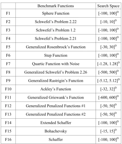
We compared the bSaM with SaM and the bSaM extended ACDE with the state-of-the-art DE algorithms in various benchmark problems. Table I. presents the problems. The following is the compared DE algorithms.
1) ACDE + bSaM with ACDE approach; 2) MDE [13];
3) jDE [3]; 4) SaDE [5];
5) Standard DE with F=0.5 and CR=0.9 [1][3];
We fixed the population size at 100 and 400 in dimension 30 and 100 experiments. All values of control parameters used in the performance evaluation were the recommended values by their authors. We executed 100 times independently to gather the results of the performance evaluation, which are the average of optimization results (MEAN) and its standard deviation (STD). To make the result clear, we marked the best result in boldface.
B. Comparison Between the Proposed Algorithm and the State-of-the-Art DE Algorithms
Table II presents the experiment result of comparison in dimension 30 experiments. The result showed that the proposed algorithm found better optimum values than the compared DE algorithms except F3, and F5. In F3, the SaDE showed best optimization performance. In F5, the standard DE showed best optimization performance. The proposed algorithm showed second best optimization performance in F3 and second best optimization performance in F5. Although the proposed algorithm performed not better in some benchmark problems, it outperformed in other benchmark problems.
Table III presents the experiment result of comparison in dimension 100 experiments. The result showed that the proposed algorithm found better optimum values than the compared DE algorithms except F3, F4, F5, F10, F15, TABLEI.
BENCHMARK FUNCTIONS
Benchmark Functions Search Space F1 Sphere Function [-100, 100]D
F2 Schwefel’s Problem 2.22 [-10, 10]D
F3 Schwefel’s Problem 1.2 [-100, 100]D
F4 Schwefel’s Problem 2.21 [-100, 100]D
F5 Generalized Rosenbrock’s Function [-30, 30]D
F6 Step Function [-100, 100]D
F7 Quartic Function with Noise [-1.28, 1.28]D
F8 Generalized Schwefel’s Problem 2.26 [-500, 500]D
F9 Generalized Rastrigin’s Function [-5.12, 5.12]D
F10 Ackley’s Function [-32, 32]D
F11 Generalized Griewank’s Function [-600, 600]D
F12 Generalized Penalized Functions #1 [-50, 50]D
F13 Generalized Penalized Functions #2 [-50, 50]D
F14 Extended Schaffer [-100, 100]D
F15 Bohachevsky [-15, 15]D
and F16. In F3 and F10, the SaDE showed best optimization performance. In F4, F5, F15, and F16, the jDE showed best optimization performance. The
proposed algorithm showed second best optimization performance in F3, F5, F15, and F16 and third best optimization performance in F4 and fifth best TABLEII.
COMPARISON BETWEEN THE PROPOSED ALGORITHM AND THE STATE-OF-THE-ART DEALGORITHMS (DIMENSION =30)
F D MAX GEN
The Proposed
Algorithm MDE jDE SaDE DE/rand/1/bin
MEAN STD MEAN STD MEAN STD MEAN STD MEAN STD F1 30 1500 1.16E-36 2.05E-36 7.54E-17 3.81E-17 1.89E-28 2.20E-28 3.36E-20 7.24E-20 6.96E-14 4.83E-14
F2 30 2000 1.05E-26 7.55E-27 5.00E-13 1.35E-13 1.65E-23 1.31E-23 6.31E-15 3.42E-15 9.55E-10 6.03E-10
F3 30 5000 3.65E-24 1.58E-23 3.67E-01 6.38E-02 2.78E-14 4.55E-14 2.37E-35 8.78E-35 3.69E-11 5.32E-11
F4 30 5000 2.47E-16 3.60E-16 2.12E-08 7.96E-09 9.10E-15 7.50E-14 8.15E-10 2.16E-10 6.95E-02 2.59E-01
F5 30 20000 1.99E-01 8.69E-01 1.20E-01 6.80E-01 1.20E-01 6.80E-01 1.33E+01 1.15E+01 1.97E-30 9.13E-30
F6 30 1500 0.00E+00 0.00E+00 0.00E+00 0.00E+00 0.00E+00 0.00E+00 0.00E+00 0.00E+00 0.00E+00 0.00E+00
F7 30 3000 2.31E-03 6.39E-04 8.53E-03 1.67E-03 3.46E-03 9.07E-04 4.31E-03 1.35E-03 4.49E-03 1.27E-03
F8 30 9000 -12569.5 1.27E-11 -11426.4 3.10E+02 -12569.5 1.27E-11 -12568.3 1.18E+01 -11143 5.15E+02
F9 30 5000 0.00E+00 0.00E+00 3.89E+01 6.16E+00 0.00E+00 0.00E+00 0.00E+00 0.00E+00 7.11E+01 2.56E+01
F10 30 1500 6.59E-15 7.07E-16 3.89E-09 8.54E-10 1.12E-14 2.54E-14 5.63E-11 3.84E-11 8.94E-08 4.24E-08
F11 30 2000 0.00E+00 0.00E+00 6.53E-03 8.35E-03 0.00E+00 0.00E+00 0.00E+00 0.00E+00 0.00E+00 0.00E+00
F12 30 1500 1.57E-32 3.56E-47 5.02E-16 2.23E-15 1.03E-29 1.18E-29 2.79E-20 4.70E-20 6.67E-15 6.29E-15
F13 30 1500 2.20E-32 4.08E-33 2.81E-17 1.43E-17 1.00E-28 1.24E-28 5.60E-20 7.88E-20 4.48E-14 3.97E-14
F14 30 1000 4.17E-22 5.61E-22 7.36E-11 4.37E-11 5.72E-17 4.92E-17 3.88E-12 4.85E-12 1.98E-07 1.44E-07
F15 30 3000 4.12E-16 2.65E-16 3.49E-05 1.22E-05 1.24E-15 6.84E-16 1.40E-07 2.82E-08 7.35E-04 7.31E-04
F16 30 1000 2.85E-22 5.08E-22 1.12E-08 5.01E-09 1.50E-16 3.06E-16 1.56E-10 1.46E-10 2.23E-05 1.57E-05
TABLEIII.
COMPARISON BETWEEN THE PROPOSED ALGORITHM AND THE STATE-OF-THE-ART DEALGORITHMS (DIMENSION =100)
F D MAX GEN
The Proposed
Algorithm MDE jDE SaDE DE/rand/1/bin
MEAN STD MEAN STD MEAN STD MEAN STD MEAN STD F1 100 2000 7.79E-22 6.78E-22 2.25E-01 2.28E-02 3.96E-15 1.39E-15 3.52E-09 3.56E-09 1.94E+01 4.53E+00
F2 100 3000 6.38E-19 5.31E-19 3.84E-01 2.22E-02 5.47E-15 1.47E-15 1.84E-06 3.95E-07 5.63E+01 2.21E+01
F3 100 8000 9.21E-08 2.21E-07 3.25E+02 4.25E+01 4.66E-02 2.49E-02 1.00E-12 3.77E-12 1.21E+05 1.65E+04
F4 100 15000 1.96E-05 1.16E-05 6.04E-01 2.79E-02 3.11E-09 5.88E-10 6.44E-06 7.10E-07 9.21E+01 1.09E+01
F5 100 20000 2.79E-01 1.02E+00 9.03E+01 2.74E+01 1.68E-01 5.87E-01 8.93E+01 1.75E+01 3.86E+01 5.25E+00
F6 100 1500 0.00E+00 0.00E+00 3.00E-01 4.80E-01 0.00E+00 0.00E+00 0.00E+00 0.00E+00 2.03E+02 3.97E+01
F7 100 6000 2.57E-03 4.15E-04 2.42E-01 2.16E-02 7.98E-03 1.02E-03 9.44E-03 3.68E-03 2.71E-02 4.69E-03
F8 100 9000 -41898.3 6.55E-11 -40479.8 3.81E+02 -41898.3 6.55E-11 -41898.3 6.55E-11 -12810.1 1.07E+03
F9 100 9000 0.00E+00 0.00E+00 5.13E+02 2.23E+01 0.00E+00 0.00E+00 0.00E+00 0.00E+00 8.05E+02 1.70E+01
F10 100 3000 7.18E-01 5.64E-01 4.88E-02 3.51E-03 3.95E-08 2.80E-07 3.80E-08 1.80E-08 7.11E-01 3.39E+00
F11 100 3000 0.00E+00 0.00E+00 2.39E-03 4.92E-03 0.00E+00 0.00E+00 4.49E-14 2.27E-13 1.24E-01 3.19E-02
F12 100 3000 3.49E-32 1.47E-32 1.98E-04 9.11E-05 7.92E-26 4.08E-26 9.20E-14 7.45E-14 3.46E-02 2.00E-02
F13 100 3000 1.47E-31 2.41E-32 4.88E-03 6.69E-04 8.93E-25 5.81E-25 1.34E-13 8.65E-14 5.29E-01 2.10E-01
F14 100 1000 3.30E-04 1.87E-03 1.14E+00 1.01E-01 9.66E-04 3.05E-04 2.86E-02 1.86E-02 1.02E+07 4.52E+06
F15 100 3000 1.67E+00 1.90E-01 5.41E+01 1.92E+00 1.69E-04 3.60E-05 3.72E+00 2.09E-01 4.18E+01 3.16E+00
optimization performance in F10. Similar to the dimension 30 experiments, although the proposed TABLEIV.
COMPARISON BETWEEN BSAM WITH ACDEPARAMETER ADAPTATION AND THE SAM WITH JADEPARAMETER ADAPTATION
F D MAX GEN
ACDE+bSaM with ACDE approach
ACDE+SaM with JADE approach MEAN STD MEAN STD F1 30 1500 1.16E-36 2.05E-36 6.64E-34 1.21E-33
F2 30 2000 1.05E-26 7.55E-27 3.90E-24 2.75E-24
F3 30 5000 3.65E-24 1.58E-23 8.70E-29 2.79E-28
F4 30 5000 2.47E-16 3.60E-16 1.77E-16 5.13E-16
F5 30 20000 1.99E-01 8.69E-01 9.30E-01 1.69E+00
F6 30 1500 0.00E+00 0.00E+00 0.00E+00 0.00E+00
F7 30 3000 2.31E-03 6.39E-04 2.58E-03 6.67E-04
F8 30 9000 -12569.5 1.27E-11 -12569.5 1.82E-12
F9 30 5000 0.00E+00 0.00E+00 0.00E+00 0.00E+00
F10 30 1500 6.59E-15 7.07E-16 5.49E-14 1.03E-13
F11 30 2000 0.00E+00 0.00E+00 2.05E-03 5.28E-03
F12 30 1500 1.57E-32 3.56E-47 5.54E-32 9.61E-32
F13 30 1500 2.20E-32 4.08E-33 7.37E-32 3.56E-32
F14 30 1000 4.17E-22 5.61E-22 1.74E-19 2.73E-19
F15 30 3000 4.12E-16 2.65E-16 1.32E-14 1.65E-14
F16 30 1000 2.85E-22 5.08E-22 3.50E-02 1.88E-01
TABLEV.
COMPARISON BETWEEN BSAM WITH ACDEPARAMETER ADAPTATION AND THE SAM WITH ACDEPARAMETER ADAPTATION
F D MAXGEN
ACDE+bSaM with ACDE approach
ACDE+SaM with ACDE approach MEAN STD MEAN STD
F1 30 1500 1.16E-36 2.05E-36 2.02E-36 7.55E-36
F2 30 2000 1.05E-26 7.55E-27 2.43E-26 1.95E-26
F3 30 5000 3.65E-24 1.58E-23 1.96E-26 6.59E-26
F4 30 5000 2.47E-16 3.60E-16 1.12E-17 6.85E-18
F5 30 20000 1.99E-01 8.69E-01 6.78E-01 1.50E+00
F6 30 1500 0.00E+00 0.00E+00 0.00E+00 0.00E+00
F7 30 3000 2.31E-03 6.39E-04 2.46E-03 7.20E-04
F8 30 9000 -12569.5 1.27E-11 -12569.5 1.27E-11
F9 30 5000 0.00E+00 0.00E+00 0.00E+00 0.00E+00
F10 30 1500 6.59E-15 7.07E-16 3.77E-14 7.53E-14
F11 30 2000 0.00E+00 0.00E+00 6.41E-04 2.22E-03
F12 30 1500 1.57E-32 3.56E-47 1.57E-32 3.56E-47
F13 30 1500 2.20E-32 4.08E-33 1.43E-32 1.44E-33
F14 30 1000 4.17E-22 5.61E-22 2.28E-22 4.28E-22
F15 30 3000 4.12E-16 2.65E-16 1.12E-14 8.00E-15
F16 30 1000 2.85E-22 5.08E-22 4.11E-22 1.49E-21
TABLEVI.
COMPARISON BETWEEN BSAM WITH ACDEPARAMETER ADAPTATION AND THE BSAM WITH JADEPARAMETER ADAPTATION
F D MAX GEN
ACDE+bSaM with
ACDE approach ACDE+bSaM with JADE approach MEAN STD MEAN STD F1 30 1500 1.16E-36 2.05E-36 6.70E-35 1.96E-34
F2 30 2000 1.05E-26 7.55E-27 4.87E-26 6.43E-26
F3 30 5000 3.65E-24 1.58E-23 1.32E-17 1.31E-16
F4 30 5000 2.47E-16 3.60E-16 4.06E-15 7.78E-15
F5 30 20000 1.99E-01 8.69E-01 7.97E-02 5.58E-01
F6 30 1500 0.00E+00 0.00E+00 0.00E+00 0.00E+00
F7 30 3000 2.31E-03 6.39E-04 2.52E-03 6.07E-04
F8 30 9000 -12569.5 1.27E-11 -12569.5 1.27E-11
F9 30 5000 0.00E+00 0.00E+00 0.00E+00 0.00E+00
F10 30 1500 6.59E-15 7.07E-16 8.01E-15 2.79E-15
F11 30 2000 0.00E+00 0.00E+00 0.00E+00 0.00E+00
F12 30 1500 1.57E-32 3.56E-47 1.57E-32 1.28E-34
F13 30 1500 2.20E-32 4.08E-33 3.77E-32 5.71E-33
F14 30 1000 4.17E-22 5.61E-22 2.54E-21 3.71E-21
F15 30 3000 4.12E-16 2.65E-16 9.08E-16 8.98E-16
F16 30 1000 2.85E-22 5.08E-22 1.37E-21 1.45E-21
TABLEVII.
COMPARISON BETWEEN THE LONG-TAILED AND THE SHORT-TAILED
DISTRIBUTIONS FOR THE BSAM
F D MAXGEN
Cauchy Distribution
For bSaM Gaussian DistributionFor bSaM MEAN STD MEAN STD
F1 30 1500 1.16E-36 2.05E-36 1.73E-34 2.42E-34
F2 30 2000 1.05E-26 7.55E-27 3.17E-25 4.58E-25
F3 30 5000 3.65E-24 1.58E-23 8.94E-25 7.45E-24
F4 30 5000 2.47E-16 3.60E-16 3.55E-15 1.36E-14
F5 30 20000 1.99E-01 8.69E-01 2.79E-01 1.02E+00
F6 30 1500 0.00E+00 0.00E+00 0.00E+00 0.00E+00
F7 30 3000 2.31E-03 6.39E-04 2.58E-03 8.31E-04
F8 30 9000 -12569.5 1.27E-11 -12569.5 1.27E-11
F9 30 5000 0.00E+00 0.00E+00 0.00E+00 0.00E+00
F10 30 1500 6.59E-15 7.07E-16 7.05E-15 1.73E-15
F11 30 2000 0.00E+00 0.00E+00 0.00E+00 0.00E+00
F12 30 1500 1.57E-32 3.56E-47 1.63E-32 2.11E-33
F13 30 1500 2.20E-32 4.08E-33 4.73E-32 2.52E-32
F14 30 1000 4.17E-22 5.61E-22 1.95E-18 6.81E-18
F15 30 3000 4.12E-16 2.65E-16 1.00E-14 5.66E-14
algorithm performed not better in some benchmark problems, it outperformed in other benchmark problems.
C. Comparison Between bSaM with ACDE Parameter Adaptation and the SaM with JADE Parameter Adaptation
We attempted to verify that the extended ACDE by the bSaM with ACDE approach is more useful than the extended ACDE by the SaM with JADE approach. Table IV presents the experiment result of comparison. The result showed that the extended ACDE by the bSaM with ACDE approach found better optimum values than the extended ACDE by the SaM with JADE approach except F3 and F4. However, in F1, F2, F10, F11, F14, F15, and F16, the extended ACDE by the bSaM with ACDE approach found much better optimum values. As a result, the extended ACDE by the bSaM with ACDE approach can find better optimum values than the extended ACDE by the SaM with JADE approach in various problems.
D. Comparison Between bSaM with ACDE Parameter Adaptation and the SaM with ACDE Parameter Adaptation
We attempted to verify that the extended ACDE by the bSaM with ACDE approach is more useful than the extended ACDE by the SaM with ACDE approach. Table V presents the experiment result of comparison. The result showed that the extended ACDE by the bSaM with ACDE approach found better optimum values than the extended ACDE by the SaM with ACDE approach except F3, F4, F13, and F14. However, the differences of F13,
and F14 were not significant and in F10, F11, F15 and F16, the extended ACDE by the bSaM with ACDE approach algorithm found much better optimum values. As a result, the extended ACDE by the bSaM with ACDE approach can find better optimum values than the extended ACDE by the SaM with ACDE approach in various problems.
E. Comparison Between bSaM with ACDE Parameter Adaptation and the bSaM with JADE Parameter Adaptation
We attempted to verify that the extended ACDE by the bSaM with ACDE approach is more useful than the extended ACDE by the bSaM with JADE approach. Table VI presents the experiment result of comparison. The result showed that the extended ACDE by the bSaM with ACDE approach found better optimum values than the extended ACDE by the bSaM with JADE approach except F5. However, in F1, F3, F4, F14, and F16, the extended ACDE by bSaM with ACDE approach found much better optimum values. As a result, the extended ACDE by the bSaM with ACDE approach can find better optimum values than the extended ACDE by the bSaM with JADE approach in various problems.
F. Comparison Between the Long-tailed and the Short-tailed Distributions for the bSaM
We attempted to verify that the Lang-tailed distribution is more useful than the Short-tailed distribution in terms of the strategy adaptation of the bSaM with ACDE approach. Table VII presents the experiment result of TABLEVIII.
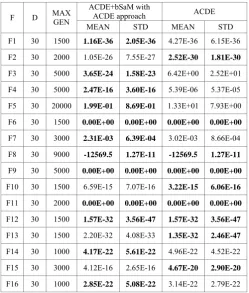
COMPARISON BETWEEN THE EXTENDED ACDE BY BSAM WITH ACDE PARAMETER ADAPTATION WITH THE ACDE(DIMENSION =30)
F D MAX GEN
ACDE+bSaM with
ACDE approach ACDE
MEAN STD MEAN STD F1 30 1500 1.16E-36 2.05E-36 4.27E-36 6.15E-36
F2 30 2000 1.05E-26 7.55E-27 2.52E-30 1.81E-30
F3 30 5000 3.65E-24 1.58E-23 6.42E+00 2.52E+01
F4 30 5000 2.47E-16 3.60E-16 5.39E-06 5.37E-05
F5 30 20000 1.99E-01 8.69E-01 1.33E+01 7.93E+00
F6 30 1500 0.00E+00 0.00E+00 0.00E+00 0.00E+00
F7 30 3000 2.31E-03 6.39E-04 3.02E-03 8.66E-04
F8 30 9000 -12569.5 1.27E-11 -12569.5 1.27E-11
F9 30 5000 0.00E+00 0.00E+00 0.00E+00 0.00E+00
F10 30 1500 6.59E-15 7.07E-16 3.22E-15 6.06E-16
F11 30 2000 0.00E+00 0.00E+00 0.00E+00 0.00E+00
F12 30 1500 1.57E-32 3.56E-47 1.57E-32 3.56E-47
F13 30 1500 2.20E-32 4.08E-33 1.35E-32 2.46E-47
F14 30 1000 4.17E-22 5.61E-22 4.96E-22 4.52E-22
F15 30 3000 4.12E-16 2.65E-16 4.67E-20 2.90E-20
F16 30 1000 2.85E-22 5.08E-22 3.14E-22 2.79E-22
TABLEIX.
COMPARISON BETWEEN THE EXTENDED ACDE BY BSAM WITH ACDE PARAMETER ADAPTATION WITH THE ACDE(DIMENSION =100)
F D MAXGEN
ACDE+bSaM with
ACDE approach ACDE
MEAN STD MEAN STD
F1 100 2000 7.79E-22 6.78E-22 2.24E-19 7.18E-20
F2 100 3000 6.38E-19 5.31E-19 2.61E-19 5.48E-20
F3 100 8000 9.21E-08 2.21E-07 2.49E+01 1.80E+01
F4 100 15000 1.96E-05 1.16E-05 7.29E-06 7.86E-07
F5 100 20000 2.79E-01 1.02E+00 1.03E+02 2.18E+01
F6 100 1500 0.00E+00 0.00E+00 0.00E+00 0.00E+00
F7 100 6000 2.57E-03 4.15E-04 6.21E-03 1.21E-03
F8 100 9000 -41898.3 6.55E-11 -41898.3 6.55E-11
F9 100 9000 0.00E+00 0.00E+00 0.00E+00 0.00E+00
F10 100 3000 7.18E-01 5.64E-01 1.21E-09 2.18E-09
F11 100 3000 0.00E+00 0.00E+00 0.00E+00 0.00E+00
F12 100 3000 3.49E-32 1.47E-32 1.32E-30 5.64E-31
F13 100 3000 1.47E-31 2.41E-32 2.68E-30 1.18E-30
F14 100 1000 3.30E-04 1.87E-03 1.91E-05 5.26E-06
F15 100 3000 1.67E+00 1.90E-01 3.38E-04 1.20E-04
comparison. We applied the Cauchy and Gaussian distributions as the Long-tailed and the Short-tailed distributions to the strategy adaptation of the bSaM. The result showed that the Long-tailed distribution found better optimum values than the Short-tailed distribution except F3. However, in F1, F2, F4, F14, F15, and F16, the Long-tailed distribution found much better optimum values. As a result, the Long-tailed distribution performs better than the Short tailed distribution for adapting the strategy parameter of the bSaM.
G. Comparison Between the Extended ACDE by bSaM with ACDE Parameter Adaptation with the ACDE
Table VIII presents the experiment result of comparison in dimension 30 experiments. The result showed that the extended ACDE by bSaM with ACDE approach found better optimum values than the ACDE except F2, F4, F10, F14, F15, and F16. However, the differences of F10 and F13 ware not significant and in F3, F4, and F5, the extended ACDE by the bSaM with ACDE approach found much better optimum values.
Table IX presents the experiment result of comparison in dimension 100 experiments. The result showed that the extended ACDE by bSaM with ACDE approach found better optimum values than the ACDE except F2, F4, F10, F15, and F16. However, the difference of F2 was not significant and in F1, F3, F5, F7, F12, and F13, the extended ACDE by the bSaM with ACDE approach found much better optimum values.
As a result, the extended ACDE by the bSaM with ACDE approach can find better optimum values than the ACDE in various problems.
V. CONCLUSION
In this paper, we modified the SaM for strictly controlling a balance between the exploration and the exploitation properties, which called the bSaM. We extend the ACDE to attach the bSaM. The performance evaluation showed that the bSaM performed better than the SaM and the ACDE’s adaptive parameter control performed better than the JADE’s adaptive parameter control in terms of adapting the strategy probability. In addition, we found out that the Long-tailed distribution still performs better than the Short-tailed distribution for the bSaM.
REFERENCES
[1] R. Storn and K. Price, “Differential evolution a simple and efficient heuristic for global optimization over continuous spaces,” Journal of Global Optimization, vol. 11, Issue 4, pp. 341-359, December 1997.
[2] S. Das and P. N. Suganthan, “Differential evolution: A survey of the State-of-the-Art,” Evolutionary Computation, IEEE Transactions on, vol. 15, Issue 1, pp. 4-31, February
2011.
[3] J. Brest, S. Greiner, B. Bošković, M. Mernik, and V. Žumer, “Self-adapting control parameters in differential evolution: A comparative study on numerical benchmark problems,” Evolutionary Computation, IEEE Transactions on, vol. 10, Issue 6, pp. 646-657, December 2006.
[4] A. E. Eiben and J. E. Smith, Introduction to Evolutionary Computing, Berlin, Germany: Springer-Verlag, 2003. [5] A. K. Qin and P. N. Suganthan, “Self-adaptive differential
evolution algorithm for numerical optimization,” in Proc. Evolutionary Computation, 2005, The 2005 IEEE Congress on, vol. 2, September 2005, pp. 1785-1791.
[6] J. Brest, B. Bošković, S. Greiner, V. Žumer, and M. S. Maučec, “Performance comparison of self-adaptive and adaptive differential evolution algorithms,” Soft Computing,
vol. 11, Issue 7, pp 617-629, May 2007.
[7] J. Zhang and A. C. Sanderson, “JADE: Adaptive differential evolution with optional external archive,”
Evolutionary Computation, IEEE Transactions on, vol. 13,
Issue 5, pp. 945-958, October 2009.
[8] W. Gong, Z. Cai, C. X. Ling, and H. Li, “Enhanced differential evolution with adaptive strategies for numerical optimization,” Systems, Man, And Cybernetics-Part B: Cybernetics, IEEE Transactions on, vol. 41, Issue 2, pp.
397-413, April 2011.
[9] A. K. Qin, V. L. Huang, and P. N. Suganthan, “Differential evolution algorithm with strategy adaptation for global numerical optimization,” Evolutionary Computation, IEEE Transactions on, vol. 13, Issue 2, pp. 398-417, April 2009.
[10]T. J. Choi, C. W. Ahn, and J. An, “An adaptive cauchy differential evolution algorithm for global numerical optimization,” The Scientific World Journal, vol. 2013, Article ID 969734, 12 pages, 2013. doi:10.1155/2013/969734
[11]J. Brest and M. S. Maučec, “Population size reduction for the differential evolution algorithm,” Applied Intelligence,
vol. 29, Issue 3, pp. 228-247, December 2008.
[12]J. Teo, “Exploring dynamic self-adaptive populations in differential evolution,” Soft Computing, vol. 10, no. 8, pp.
673–686, 2006.
[13]M. Ali and M. Pant, “Improving the performance of differential evolution algorithm using Cauchy mutation,” Soft Computing, vol. 15, Issue 5, pp. 991-1007, May 2011.
Tae Jong Choi received M.S at the
Department of Computer Engineering, Ajou University, Republic of Korea. He is currently working toward Ph.D. degree at the Department of Computer Engineering, Sungkyunkwan University (SKKU), Republic of Korea. His research interests include genetic algorithms and the applications of evolutionary techniques to wireless networks.
Chang Wook Ahn received Ph.D.