Effect of Cutting Parameters on Drilling to
Optimize MRR and Temperature by Response
Surface Methodology under Dry Condition
B. Pradeep Kumar
#1, J. V. Bhanutej
#2, Dr. B. NagaRaju
#3(Size 11)
#1,2 Assistant Professor, #3Professor & Department of Mechanical Engineering, ANITS.
sangivalsa-531162, Vishakhapatnam dist. Andhra Pradesh, India.
Abstract The main objective of this work deals with the effect of cutting parameters on EN8(080M40) carbon steel specimen in drilling operation to optimize the minimum temperature and maximum material removal rate using surface response analysis. Now a days EN8 is used in many engineering applications such as manufacturing of shafts, gears, stressed pins, studs, bolts, keys etc., due to its good tensile strength. In the present work full factorial design is considered with process parameters such as speed, feed , diameter of drill bit . By using mathematical model the main and interaction effect of various process parameters on MRR and temperature is studied. The developed model helps in selection of proper machining parameters for specific material and helps in achieving desired material removal rate and minimum temperature under dry condition.
Keywords— EN8, MRR., Temperature.
I. INTRODUCTION
1.1 Drilling Operation
Drilling is a cutting process that uses a drill bit to cut a hole of circular cross-section in solid materials. The drill bit is usually a rotary cutting tool, often multipoint. The bit is pressed against the workpiece and rotated at rates from hundreds to thousands of revolutions per minute. This forces the cutting edge against the workpiece, cutting off chips from the hole as it is drilled.
The machine used for drilling is called drilling machine.
The drilling operation can also be accomplished
in lathe, in which the drill is held in tailstock and the work is held by the chuck.
The most common drill used is the twist drill.
Fig1.1 Drilling Operation
1.2 Adjustable cutting parameters in drilling
The three primary factors in any basic drilling operation are speed, feed and depth of cut other factors such as kind of material and type of tool have a large influence , of course , but these three are the ones the operator can change by adjusting the controls, right on the machine
1.2.1. Speed:
Speed always refers to the spindle and the work piece. When it is stated in revolutions per minute (rpm).it defines the speed of rotation. But, the important feature for a particular Drilling operation is the surface speed, or the speed at which the work piece material is moving past the cutting tool. It is simply, the product of the rotating speed times the circumference of the work piece before the cut is started. It is expressed in meter per minute (m/min), and it refers only to the work piece. Every different diameter on a work piece will have a different cutting speed, even though the rotating speed remains the same
V=πDN/1000
Here, v is the cutting speed in Drilling in m/ min, D is the initial diameter of the workpiece in mm. N is the Drill bit speed in r.p.m.
1.2.2 Feed:
Feed always refers to the cutting tool, and it is the rate at which the tool advances along its cutting path. On most power-fed machines, the feed rate is directly related to the spindle speed and is expressed in mm (of tool advance) per revolution (of the spindle), or mm/rev.
f- Feed in mm/rev and N - Spindle speed in r.p.m.
1.2.3 Depth of Cut:
Depth of cut is practically self- explanatory .It is the thickness of the layer being oved (in a single pass) from the workpiece or the distance from the uncut surface of work to the cut surface, expressed in mm. It is important to note, though, that the diameter of the work piece is reduced by two times the depth of cut because this layer is being removed from both sides of the work
D = (D –d) / 2 D - Depth of cut in mm
D - Initial diameter of the work piece d - Final diameter of the work piece
II. EXPERIMENTATION
The present work was done in 3 stages.
Design of experiments was done using full factorial method.
Observation and calculation of cutting forces, temperature, material removal rate by machining the work piece on Radial drilling machine in both wet and dry conditions. Analysis of results was done using MINITAB 15.1.30.
2.1. Selection of process variables
A total of three process variables and 2 levels are selected for the experimental procedure.
The deciding process variables are Speed
Feed
Diameter of drill bit
Speed of the spindle, i.e. the speed at which the spindle rotates the tool.
Feed is the rate at which the material is removed from the work piece.
Diameter of drill bit is the diameter of the hole to be drilled on the work piece.
Selection of levels:
Since it is a three level design by observing the parameters taken in various projects the levels of the factors are designed as follows
Table I : Selection of process variables
Factors Level1 Level2 Speed(rpm) 180 112 Feed(mm/rev) 0.21 0.13 Diameter of drill bit(mm) 14 12
2.2. Design of Experiments
Design of experiments was done using full factorial method. Design of experiments (DOE) or experimental design is the design of any information-gathering exercises where variation is
present, whether under the full control of the experimenter or not.
The coded form in design of experiments was done by giving the values of input parameters to the MINITAB software. The coded form is given as “+1” for the maximum input and “-1” for minimum output, these are shown in Table II
Table II : Design of Experiments in coded form
Expt NO S.Speed (rpm)
Feed (mm/rev)
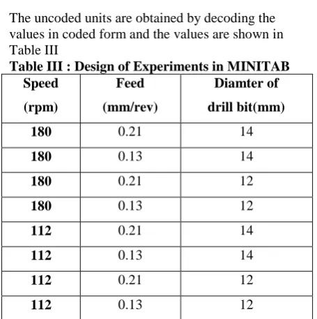
Diameter of drill bit(mm) 1 +1 +1 +1 2 +1 -1 +1 3 +1 +1 -1 4 +1 -1 -1 5 -1 +1 +1 6 -1 -1 +1 7 -1 +1 -1 8 -1 -1 -1 The uncoded units are obtained by decoding the values in coded form and the values are shown in Table III
Table III : Design of Experiments in MINITAB Speed
(rpm)
Feed
(mm/rev)
Diamter of
drill bit(mm)
180 0.21 14
180 0.13 14
180 0.21 12
180 0.13 12
112 0.21 14
112 0.13 14
112 0.21 12
112 0.13 12
2.3. Machining of the workpiece
The machining of the work piece on Radial Drilling Machine is done by using the following procedure
Selection of material Clamping of the work piece Clamping of the cutting tool Drilling of the work piece
2.4 Selection of material
of its high tensile strength. The composition of EN8 is:
Carbon- 0.36-0.44% Manganese- 0.6-1.0% Phosphorous- 0.05% Sulphur- 0.005% Silicon- 0.10-0.40 Standard: BS 970-1971
The dimensions of the workpiece used are thickness 15.5 mm*50mm dia
III.RESULTSANDDISCUSSIONS
3.1 Development of Mathematical Models
A Second -order polynomial is employed for developing the mathematical model for predicting weld pool geometry. If the response is well modelled by a linear function of the independent variables then the approximating function is the first order model as shown in Equation.
Y = + 1 x1 + 2 x2 + …._ x xx +
A mathematical regression equation is developed for cycle time in every tool path and the graphs are plotted.
0 1 0 0 1 2
k k
ii i ij i j
i i i j
Y
x
x
x x
Y is the corresponding response xi are the cutting parameters
(1,2,…….k) are code levels of quantitative process variables
The terms are the second order regression coefficients
Second term is attribute to linear effect Third term corresponds to higher order effects
Fourth term includes the interactive effects of the process parameters.
And the last term indicates the experimental error.
All the estimated coefficients were used to construct the models for the response parameter and these models were used to construct the models for the response parameter and these models were tested by applying Design of Experiments (DOE) response surface methodology.
3.2 Different Terms used in Response Surface Methodology Regression table
a. P-values: P- Values (P) are used to determine which of the effects in the model are statistically significant.
o If the p-value is less than or equal to 0.5, conclude that the effect is significant.
o If the p-value is greater than 0.5, conclude that the effect is not
b. Coefficients: Coefficients are used to construct an equation representing the relationship between the response and the factors.
c. R-squared: R and adjusted R represent the proportion of variation in the response that is explained by the model.
d. R (R-Sq) describes the amount of variation in the observed responses that is explained by the model.
e. Predicted R reflects how well the model will predict future data.
f. Adjusted R is a modified R that has been adjusted for the number of terms in the model. If we include unnecessary terms, R can be artificially high. Unlike R , adjusted R may get smaller when we add terms to the model. g. Analysis of variance table: P-values (P) are used
in analysis of variance table to determine which of the effects in the model are statistically significant. The interaction effects in the model are observed first because a significant interaction will influence the main effects. h. Estimated coefficients using un coded units i. Minitab displays the coefficients in un coded
units in addition to coded units if the two units differ.
j. For each term in the model, there is a coefficient. These coefficients are useful to construct an equation representing the relationship between the response and the factors.
3.3 Graphs Obtained
a. Histogram:
A Histogram is a graphical representation of the distribution of data. It is an estimate of the probability distribution of a continuous variable( quantitative variable) and was first introduced by Karl Pearson .The Histogram is the most commonly used graph to show frequency distributions. Histograms give a rough sense of the density of the data, and often for density estimation estimating the probability density function of the underlying variable. The total area of a histogram used for probability density is always normalised to 1.If the length of the intervals on the X-axis are all 1, then a histogram is identical to a relative frequency plot.
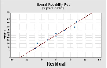
b. Normal plot of residuals:
It shows the graph plotted between the residuals versus their expected values when the distribution is normal. The residuals from the analysis should be normally distributed. In practice, for balanced ort nearly balanced designs or for data with large number of observations, moderate departures from normality do not seriously affect the results. The normal probability plot of the residuals should roughly follow a straight line.
c. Contour plots:
conditions. A contour plot provides a two-dimensional view where all points that have the same response are connected to produce contour lines of constant responses .A surface plot provides a three-dimensional view that may provide a clearer picture of the response surface.
Table IV: Response surface regression: MRR versus Speed, Feed, Dia Coded Coefficients
Term Coef SE
Coef T-
Value P-
Value VIF
Constant 27.970 0.660 42.38 0.015 0
SPEED 5.498 0.660 8.33 0.076 1.00
FEED 5.557 0.660 8.42 0.075 1.00
DIAMETER 1.600 0.660 2.42 0.249 1.00
SPEED
*FEED -0.015 0.660 -0.02 0.986 1.00
SPEED
*DIAMETER -0.468 0.660 -0.71 0.608 1.00
FEED
*DIAMETER -0.473 0.660 -0.72 0.604 1.00
Regression Equation in Un coded Units
MRR = -92.5 + 0.342 SPEED + 294 FEED + 5.62
DIAMETER0.011SPEED*FEED0.0137SPEED*DIAMETER -11.8FEED*DIAMETER
1.750 0E-1
2 1.500
0E-1 2 1.250
0E-1 2 1.000
0E-1 2
7.50 00
E-13 5.00
00 E-13 2.50
00 E-13
0.00 00E+
00
4
3
2
1
0
Residual
F
re
q
u
e
n
c
y
Histogram
(response is M RR_1)
Fig 3.1 Histogram of MRR
Fig3.2 Normal plots of Residuals as MRR
diameter 15.905 Hold Values
speed
fe
e
d
175 150
125 0.20
0.18
0.16
0.14
> – – – < 2000 2000 3000 3000 4000 4000 5000 5000 MRR_1
Contour Plot of M RR_1 vs feed, speed
Fig3.3 Contour plot of MRR
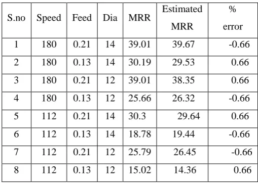
Table V: Experimental and predicted values of MRR
S.no Speed Feed Dia MRR Estimated MRR
Table VI: Response surface regression: Temperature versus Speed, Feed, Dia Coded Coefficients
Term Coef SE
Coef T-
Value P-
Value VIF
Constant 0.6987 0 0 0 0
SPEED -0.1628 0 0 0 1.00
FEED -0.1623 0 0 0 1.00
DIAMETER 0 0 0 0 1.00
SPEED
*FEED 0.0382 0 0 0 1.00
SPEED
*DIAMETER 0 0 0 0 1.00
FEED
*DIAMETER 0 0 0 0 1.00
Regression Equation in Un coded Units
TEMP = -37 + 1.203 SPEED + 726 FEED + 5.2 DIAMETER - 1.93 SPEED*FEED - 0.0684 SPEED*DIAMETER- 40.7 FEED*DIAMETER
15 10 5 0 -5 -10 -15 2.0
1.5
1.0
0.5
0.0
Residual
F
re
q
u
e
n
c
y
Histogram
(response is TEM P)
Fig 3.4 Histogram of temperature
Fig 3.5 Normal plots of Residuals as Temperature
DIAMETER 13 Hold Values
SPEED
F
E
E
D
175 150
125 0.20
0.18
0.16
0.14
> – – – – – < 58 58 60 60 62 62 64 64 66 66 68 68 TEMP
Contour Plot of TEM P vs FEED, SPEED
Fig 3.6 Contour plot of temperature
Table VII: Experimental and predicted values of Temperature
S.no Speed Feed Dia Temp Estimated temp
% Error 1 180 0.21 14 42.5 40.7263 1.77375 2 180 0.13 14 54.2 55.9738 -1.77375 3 180 0.21 12 70.2 71.9837 -1.77375 4 180 0.13 12 82.5 80.7262 1.77375 5 112 0.21 14 49.8 51.5737 -1.77375 6 112 0.13 14 58.1 56.3262 1.77375 7 112 0.21 12 75.3 73.5262 1.77375 8 112 0.13 12 70 71.7737 -1.77375
Fig 3.7 Optimization Results
starting point for the plot. This optimization plot allow to interectively changing the input variable settings to perform the senstifity analizes and possibly improve the intial solution.
The optimiztion plot as shown in figure significes the effect of each factor (columns) on the responses or composite desirebility (rows). The vertical red line on the graph represents the current factor settings. The numbers displayed at the topnof the column shows the current factor level settings(red). The horizontal blue line and numbers represents the responses for the current factor level. Minitab calculate the MRR and minimum temperature
From the optimization plot it can be said that the MRR is 58.18 mm3 /s and the minimum temperature is 42.50C obtained when tool speed is 180 rpm, feed is 0.21mm/rev ,diameter 15.9 mm.
IV.CONCLUSIONS
In the present work, Response Optimization problem has been solved by using an optimal parametric combination of input parameters such as Speed, Feed and Diameter of the drill bit.
These optimal parameters ensures in producing high surface quality turned product.
Response Surface Methodology is successfully implemented for optimizing the input parameters.
This project produces a direct equation with the combination of controlled parameters which can be used in industries to know the Value of Surface Roughness instead of machining.
The implementation of this gives direct equation in manufacturing industries
• reduces the manual effort • reduces the production cost • reduces the manufacturing time.
• Increases the quality of the product which is the ultimate goal of an industry.
Dry Condition:
Hence we conclude that the optimal solution for the MRR is 58.18 mm3 /s and the minimum temperature is 42.50C obtained when tool speed is 180 rpm, feed is 0.21mm/rev ,diameter 15.9 mm.
REFERENCES
[1]. B. P. Patel, Dr.P. M. George, Dr.V .J .Patel, “Experimental Studies on Perpendicularity of Drilling Operation using DOE”, International Journal of Advance Engineering and Research Development (IJAERD) Volume 1,Issue 3, April 2014, e-ISSN: 2348 - 4470 , print-ISSN:2348 640
[2]. Babur Ozcelika, EmelKuram, ErhanDemirbas and Emrah ¸Sik, “ Effects of vegetable-based cutting fluids on thewear in drilling”, Sadhana Vol. 38, Part 4, August 2013, pp. 687–706._c Indian Academy of Sciences
[3]. E. Kuram, B. Ozcelik, E. Demirbas, and E. Şık , “Effects of cutting fluid types and cutting parameters on surface roughness and thrust force”, Proceedings of the World
Congress on Engineering 2010 Vol II WCE 2010, June 30 - July 2, 2010, London, U.K.
[4]. Asst.Prof.J.Patel1A.Intwala,D.Patel,D. Gandhi ,N.Patel, M.Patel “Effect of cutting parameter on drilling operation for perpendicularity”, IOSR Journal of Mechanical and Civil Engineering (IOSR-JMCE) e-ISSN: 2278-1684,p-ISSN: 2320-334X, Volume 11, Issue 6 Ver. VI (Nov- Dec. 2014), PP 11-18
[5]. S.Sathiyaraj, A.Elanthiraiyan, G.Haripriya, V.Srikanth Pari “Optimisation of machining parameters for EN8 Steel through taguchi method”, Journal of Chemical and Pharmaceutical Sciences, JCHPS Special Issue 9: April 2015 , ISSN: 0974-2115
[6]. Gultekin Uzun1, Ugur Gokmen2, Hanifi Cinici1, Mehmet Turker1 “Effect of cutting parameters on the drilling of AlSi7 metallic foams” ,UDK 621.762:621.9:532.6:661.862 ISSN 1580-2949, ISSN 1580-2949 Original scientific article, MTAEC9, 51(1)19(2017), Materials and technology 51 (2017) 1, 19–24
[7]. Mr. T Bharadwaj and Mr. Thushar K T “Optimisation of process parameters in drilling EN8 steel using taguchi technique”, IJIRST –International Journal for Innovative Research in Science & Technology| Volume 3 | Issue 07 | December 2016
[8]. P.Venkataramaiah, G.Vijaya Kumar and P. Sivaiah, “Prediction and analysis of multi responses in drilling of EN8 steel under MQL using ANN-Taguchi
[9]. approach,” Elixir Mech. Engg. 47 (2012) 8790-8796 , ISSN:2229-712X
[10].S.Jayabal and U Natrajan “cutting parameters on thrust force and torque in drilling of E-glass / Polyster composites”, Indian journal of Engineering and material science Vol.17,December 2010,pp.463-470
[11].Sumesh A S , Melvin Eldho Shibu “Optimization Of Drilling Parameters For Minimum Surface Roughness Using Taguchi Method” IOSR Journal of Mechanical and Civil Engineering (IOSR-JMCE) e-ISSN2278-1684,p-ISSN: 2320-334X, PP 12-2011.
[12].Ramazan Cakırog, Adem, “Optimization of cutting parameters on drill bit temperature in drilling by Taguchi method”, Measurement, 3525-3531,2013
[13].J.K Sakhiya and L.M Rola ,” A Review on Cutting Parametrs of Drilling Operation “,International Journal of Futuristic Trends in Engineering and Technology Vol. 1 (02), 2014
[14].Navanth1 , T. Karthikeya Sharma ,” A study of Taguchi method based optimization of drilling parameter in dry drilling of Al alloy at low speeds”, International Journal of Engineering Sciences & Emerging Technologies, ISSN: 2231 – 6604 Volume 6, Issue 1, pp: 65-75 (2013).
[15].Erol Kilickap & Mesut Huseyinoglu & Ahmet Yardimeden, “Optimization of drilling parameters on surface roughness in drilling of AISI 1045 using response surface methodology and genetic algorithm,” Int J Adv Manuf Technol (2011) 52:79–88, DOI 10.1007/s00170-010-2710-7.
[16].J.Patel, A.Intwala, D.Patel, D.Gandhi, N.Patel and M.Patel, “A Review Article on Effect of Cutting Parameter on Drilling Operation for Perpendicularity”,
[17].IOSR Journal of Mechanical and Civil Engineering (IOSR-JMCE) ,p-ISSN: 2320-334X, Volume 11, Issue 6 Ver. VI (Nov- Dec. 2014), pp 11-18.
[18].Mr. Nalawade P.S et.al, “Cutting Parameter Optimization for Surface Finish and Hole Accuracy in Drilling Of EN-31, IOSR Journal of Mechanical and Civil Engineering (IOSR-JMCE), e-ISSN: 2278-1684,p-ISSN: 2320-334X, Volume 12, Issue 1 Ver. I, Jan- Feb. 2015, pp.20-27