Load Flow Solution of the Tanzanian Power Network Using Newton-Raphson Method and MATLAB Software

Published online December 05, 2014 (http://www.sciencepublishinggroup.com/j/ijepe) doi: 10.11648/j.ijepe.20140306.11

ISSN: 2326-957X (Print); ISSN: 2326-960X (Online)

Load flow solution of the Tanzanian power network using

Newton-Raphson method and MATLAB software

Mashauri Adam Kusekwa

Electrical Engineering Department, Dar es Salaam Institute of Technology (DIT), Dar es Salaam, Tanzania

Email address:

[email protected], [email protected]

To cite this article:

Mashauri Adam Kusekwa. Load Flow Solution of the Tanzanian Power Network Using Newton-Raphson Method and MATLAB Software. International Journal of Energy and Power Engineering. Vol. 3, No. 6, 2014, pp. 277-286. doi: 10.11648/j.ijepe.20140306.11

Abstract:

Load flow studies are the backbone of power system analysis and design. They are necessary for planning, operation, optimal power flow and economic scheduling and power exchange between utilities. This paper describes modelling procedure and present models of system components used in performing load flow analysis. The developed models are joined together to form a system network representing an approximate Tanzanian power network model. A load flow problem is formulated using the model and a MATLAB program developed using Newton-Raphson algorithm is applied in solving the problem. Simulation results are presented and analysed. The results indicate that the voltage magnitude and voltage phase angle profiles are within the operating limits of the system; it means that the selection of system components and modelling process is appropriate and accurate. The results will form the basis of other critical power system studies of the network in the future such as power system state estimation, optimal power flow and security constrained optimal power flow studies.

Keywords:

System Component Modelling, Power System, Load Flow Analysis, Newton-Raphson Method, MATLAB Software

1. Introduction

The aim of load flow analysis program [1-5] is to determine the steady-state operating condition of the power system for a given load distribution. The steady-state of a power system may be determined by finding out of real and reactive power throughout the system network and the voltage magnitude and voltage angle at all buses of the network.

The planning and day-to-day operation of modern power systems call for numerous load flow analysis. Information obtained from the analysis is useful in finding component or circuit loadings, bus voltages, real and reactive power flows, transformer tap settings, system losses, exciter voltage set points, and performance under emergency conditions. The load flow model also forms the basis for other types of analysis such as short circuit, angle and voltage stability, motor starting and harmonic studies.

Load flow problem is basically involves the solution of a set of non-linear equations for real and reactive powers at each bus. Several methods have been developed and successfully applied in solving the problem [6-9]. Methods [8-9] are derived from the Newton-Raphson method given in

[6]. Method [6] is applied in this paper. The problem to be solved is that of computing the steady-state load flow through different transmission components i.e. computing the voltage magnitude and voltage angle at all buses, real and reactive power flows and losses in the system. In this way a simplified modelling through which the whole generation-transmission-consumption system can be rapidly simulated is adopted.

The first simplification is by considering only the electrical

variables with angular frequency corresponding to

In this paper, system components from the Tanzanian power network are used in the modelling process. Load flow analysis is implemented under MATLAB environment using Newton-Raphson algorithm. The objective of the study is to develop alternative load flow software to PSS/E, which is used by the Tanzania Electric Supply Company Limited (TANESCO) at the moment.

The structure of the paper is as follows. Section 2 presents a brief account of Tanzanian power network status (generation and high voltage transmission). Section 3 presents material and method that include system component modelling procedures and developed models for load flow analysis is given. Section 4 presents overall system network modelling. Formulation of load flow problem using Newton-Raphson method and its solution algorithm is given in section 5. Section 6 presents input data, algorithm, simulation procedures and results. Section 7 discusses the obtained results, and section 8 concludes the paper.

2. Tanzanian Power Network

2.1. Generation

The Tanzanian power network comprises of hydro, thermal and gas plants [10]. The hydro system is comprised of 6 plants with a total nameplate of 561MW (see Table 1). The installed capacity of thermal generating plants totals 453.6MW (see Table 2). The installed capacity of isolated thermal generating plants totals 33.80MW. Currently, the total nameplate capacity is 1,053.05 MW. Coal power generation is between 4 to 6 MW; import of power is about 5 and 10 MW of bulk power from Uganda and 3 MW from Zambia. The demand of electricity in Tanzania which is a large country (950,000 square kilometres) is however growing at a relatively fast rate. While the annual average growth rate between 1990 and 1998 was 4.45 percent, the average load growth rate between 2003 and 2006 has been above 8 percent [11]

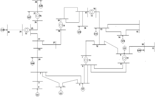
KEY: G-Generating plant, T-Two winding transformer

Figure 1. One-line diagram-Tanzanian Power Network (not to scale)

Table 1. Installed hydro grid generation capacity

Plant Name Fuel Type Installed Capacity [MW] Ownership Kihansi Hydro 180.00 TANESCO Kidatu Hydro 204.00 TANESCO Mtera Hydro 80.00 TANESCO

NPF Hydro 68.00 TANESCO

Hale Hydro 21.00 TANESCO

NYM Hydro 08.00 TANESCO

TOTAL 561.00

Figure 1. The interconnected system consists of hydro and thermal generating plants providing power to cities, Municipals and townships.

2.2. High Voltage Transmission Network

TANESCO owns high voltage and low voltage transmission and distribution lines of different voltage levels scattered all over the country. The high voltage transmission lines are estimated to comprise of 2,624.36 km of system voltage 220 kV; 1,441.50 km of 132 kV and 486.00 km of 66 kV, totalling to 4,551.86 km by the end of December 2006 [12]. High voltage transmission lines use pylons made of steel. Almost of all HV transmission lines are radial single circuit lines. The country power system is alternating current (AC) and the system frequency is 50 Hz. The TANESCO grid comprises of: South-West grid, North-West grid and North-East grid. South-East grid is still under planning stage.

South-West grid mostly of 220 kV connects: Ubungo-Morogoro-Kidatu-Kihansi-Iringa-Mufindi-Mbeya.

North-West grid connects: Ubungo-Morogoro-Kidatu-Kihansi-Iringa-Mtera-Dodoma-Singida-Shinyanga-Mwanza (220 kV); Mwanza- Musoma (132 kV)-Shinyanga- Tabora (132 kV)

North-East grid connects: Ubungo-Tegeta-Zanzibar (132 kV); Ubungo-Chalinze- Hale-NPF-Tanga (132 kV); Chalinze – Moshi – Arusha (132 kV); NYM – Moshi (66 kV); Arusha-Babati-Singida (220 kV).

Table 2. Installed thermal grid generation capacity

Plant Name Fuel Type Installed Capacity [MW] Ownership Songas Natural gas 202.00 Private Ubungo Natural gas 102.00 TANESCO

IPTL HFO 103.00 Private

Dodoma IDO 07.44 TANESCO

Mbeya IDO 13.90 TANESCO

Mwanza IDO 12.50 TANESCO

Musoma IDO 02.56 TANESCO

Tabora IDO 10.20 TANESCO

TOTAL 453.60

Source: Economic Survey Report: 2007 and2009 IDO – Industrial Diesel Oil

HFO- Heavy Fuel Oil

3. Materials and Methods

The data used for this study were obtained from TANESCO, Ubungo power station. Computer software programmed using MATLAB 2013 were used in conducting the simulation.

3.1. Modelling of System Components

A state of a power system is defined by its topology i.e. by the list of components in operation at the time of analysis and by the connections between these components. In the load-flow analysis, the system is represented in the nodal topology. The nodal topology can be defined by a graph, the buses of which are electrical buses and branches of which are the transmission system components (lines, cables, transformers).

Models of these components are presented in the following subsections.

3.2. AC synchronous Generator

Two approaches are possible for modelling AC synchronous generators: representing in detail the excitation control system or using approximate models. In system studies where system alternatives must be explored in detail, or when developing protection schemes and operating criteria to maintain the power system stability, accurate modelling is necessary and requires detailed generator models. But in the initial stages of a planning study or in operating studies such as load-flow, simplified models may be adequate for real-time determination of operating limits and for some contingency analysis studies [13]. Thus, the AC synchronous generator is modelled as a voltage-controlled bus with constant real power and voltage.

3.3. Transmission Lines

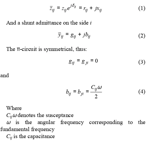
A transmission line or a cable connecting two buses (Figure 1) i and j is modelled by a π- circuit with series impedance:

ij ij j ij

ij z e r jx

z = δij = + ₍₁₎

And a shunt admittance on the side i

ij ij

ij g jb

y = + ₍₂₎

The π-circuit is symmetrical, thus:

0 = = ji ij g

g (3)

and

2

ω ij ji ij

C b

b = = (4)

Where

Cijω denotes the susceptance

ω is the angular frequency corresponding to the

fundamental frequency

Cij is the capacitance

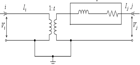
3.4. Regulating Transformer (RT)

Regulating transformers can be used to control real and reactive power flows in a circuit [14].Regulating transformers (RT) can also be used for control of voltage magnitude as well as phase angle. Thus, it is necessary to develop bus admittance equations that can be included in load flow analysis from regulating transformers. Figure 2 shows a detailed representation of a practical regulating transformer.

respectively

Figure 2. Transmission line representation

∗ = i i i VI

S (5)

∗ = i j j tVI

S (6)

Assuming the ideal transformer has no losses, the power Si

into the ideal transformer from bus i must equal the power –

Sj out of the ideal transformer on the bus j side, so from (5) and (6) ∗ ∗ ∗ − = − = − = j i j i i i j i tI I I tV I V S S (7)

The current Ij can be expressed by

Y V tYV Y tV V I j i i j j + − = − =( ) (8)

Multiplying (8) by -t• and substituting Ii for -t•Ij yield:

j i i ttYV t YV

I = ∗ − ∗ (9)

Setting tt• = t2 and re- arranging (8) and (9) into Ybus admittance matrix form, gives

              − − =       ∗ j i j i V V Y tY Y t Y t I I 2 (10)

The π-equivalent model corresponding to (10) is presented

in Figure 3.

Figure 3. Detailed representation of RT

Figure 4. π-equivalent model of RT

3.5. Loads

It has been suggested [15] that the actual load be modelled as linear combination of constant load, constant current and

constant impedance. This approach would require

considerable knowledge of load composition or knowledge of real and reactive power variation with voltage magnitude. In real power system, load models are categorized as static models or dynamic models. Static models normally express the characteristic of the load at any instant of time as algebraic function of the bus voltage magnitude and frequency at that instant time. In this way the real power

component P and the reactive power component Q are

considered separately. The load characteristic in terms of voltage for static loads is represented by exponential model:

a V V P P _      = 0

0 (11)

b V V Q Q _      = 0

0 (12)

Where

P and Q are real and reactive components of the load when

the load voltage magnitude is V. Subscript “0” identifies the values of the respective variables at the initial operating conditions

The parameters for static load the exponents “a” and “b”.

When these exponents are equal to 0, 1, 2 [15] the static load model represents constant power, constant current or constant impedance characteristic, respectively. In case of composite load, their parameter values depend on the aggregate characteristics of load components. In this study static model type of loads is adopted.

4. System Network Modelling

Given a bus load and specified voltage magnitudes/power injections at generation buses, usually conventional load flow analysis determines the steady-state operating condition of a power system based on the bus/branch network model. Such a network model is produced by merging adjacent substation buses present at the actual bus-section level topology.

or branch equations. The nodal equations for an N-bus network are the real and reactive power injections at each bus, given by [16-17].

(

)

N i B G V V P N j ij ij ij ij j i i , 1 sin cos 1 = + =

∑

= δ δ (13)

(

)

N i B G V V Q N j ij ij ij ij j i i , 1 cos sin 1 = − =

∑

= δ δ (14) where j i ij

δ

δ

δ

∆ −

:

, j

i V

V _{voltage magnitudes at buses i and j}

:

, j

i δ

δ bus voltage angles at buses i and j

:

i

P real power injection at bus i

:

i

Q reactive power injection at bus i

:

ij ij B

G + _{entry (i, j) of the nodal admittance matrix}

The branch equations provide the real and reactive power flows through the branches of the network, which are respectively, given by [17]

(

ij ij ij ij

)

i ij

j i

ij VV G B V G

P = cos

δ

+ sin

δ

− 2 (15)

(

)

(

shunt

)

ij ij i ij ij ij ij j i

ij VV G B V B b

Q = sin

δ

− cos

δ

+ 2 − (16)

where :

ij

P real power flow through branch i – j

:

ij

Q reactive power flow through branch i – j

:

Shunt ij

b shunt susceptance of branch i - j

Equations (15) and (16) can be extended to represent the power flow through tap-changing and phase-shifting transformers as given in [15]. Power injections given by (13) and (14) can also be written as the sum of the real power flow through the branches incident to bus p that is given in [15]

(

)

i j N i V V P P i j j i j i ij i ≠ = =

∑

Ω ∈ , , 1 , , , δ δ (17)

(

)

i j N i V V Q V b Q i j j i j i ij i shunt i i ≠ = + − =

∑

Ω ∈ , , 1 , ,

2 _δδ

(18)

where Ω_i:Set of buses adjacent to bus i (bus i not includes)

:

shunt i

b Shunt susceptance at bus i

5. Load Flow Problem Formulation

The load flow problem is formulated as a set of non-linear algebraic equations, normally represented by (13) and (14) and a set of inequality relationship to take into account operating limits such as reactive power injections/voltage magnitudes at generation buses. The problem solvability is

guaranteed by the classical bus classifications:

Slack/reference bus (V-δ), voltage-controlled/regulated buses

(P-V) and load buses (P-Q) [16] and [18]. Load flow usually defines a single bus i.e. reference bus, which plays a double function: it provides the phase reference angle, and since the transmission losses are unknown in advance, this bus is used to balance generation losses and load [15] and [18].

Consider an electrical power system (the Tanzanian system)

comprising of nL buses, nPV generation buses and one

reference bus. The vector of state variables i.e. voltage magnitudes and phase angles determined by the load flow formulation is given by:

[

T T

]

V

x= ,δ (19)

where

(

nL,nPV

)

=

δ Vector of phase angles

L n

V = Vector of voltage magnitudes

The set of equality equations, which represents the system of power flow problem, is given by [18-19]

( )

( )

0

, , ) ( =      − − =       ∆ ∆ = δ_δ V Q Q V P P Q P x f Sch Sche (20) where

∆P and ∆Q is the real and reactive vector of power

mismatches, respectively

Psche and Qsche the vectors of scheduled values of real and reactive power injections, respectively

P and Q are vectors of non-linear equations of real and reactive power injections, represented in equations (15) and (16), respectively

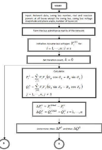
5.1. Load Flow Solution Using Newton-Raphson Method

The following linear system is generated when applying Newton-Raphson method to solve eqn (20) [5], [14], [18], [19] and [20-21]:

( )

k k k V x J Q P       ∆ ∆ =       ∆ ∆ δ (21) where

k: the iteration counter

J (xk): the problem’s Jacobian matrix given by

If m buses of the system are PV, m equations involving ∆Q

and ∆V and the corresponding column of the Jacobian matrix

are eliminated because for PV buses, the voltage magnitudes

are known. Accordingly, there are n-1 real power constrains

and (n-1-m) reactive power constraints, and the Jacobian

matrix is of order (2n-2-m) x (2n-2-m).

J1 is of the order (n-1) x (n-1)

J2 is of the order (n-1) x (n-1-m)

J3 is of order the (n-1-m) x (n-1)

J4 is of the order (n-1-m) x (n-1-m)

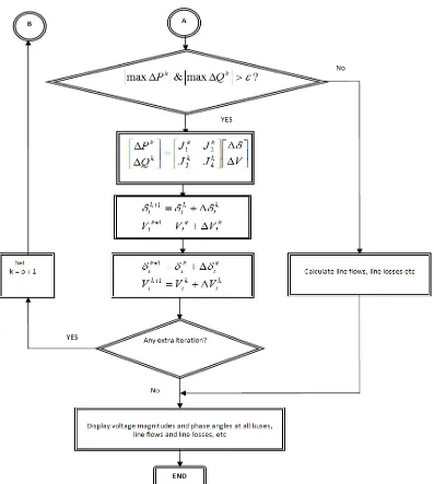
The load flow solution can be iteratively obtained by solving the linear system represented in Eqn (21). The voltage magnitudes and phase angles are updated as:

V V Vk k

k k

∆ + =

∆ + = + +

1

1 _{δ δ}

δ

(23)

Until convergence is obtained

The procedure for load flow solution by the Newton-Raphson method is given in flow chart of Figure 5.

6. Results

6.1. Input Data

Input data for load flow simulation are given in Tables 3 and 4. Table 3 gives the transmission lines of the Tanzanian Network while Table 4 provides power generation and demand of all buses in the system.

6.2. Simulation

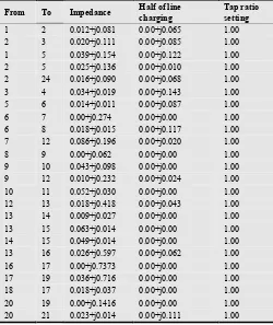
Table 3. Linedata 30-Bus Tanzania System Network

From To Impedance Half of line charging

Tap ratio setting 1 2 0.012+j0.081 0.00+j0.065 1.00 2 3 0.020+j0.111 0.00+j0.085 1.00 1 5 0.039+j0.154 0.00+j0.122 1.00 2 5 0.025+j0.136 0.00+j0.010 1.00 2 24 0.016+j0.090 0.00+j0.068 1.00 3 4 0.034+j0.019 0.00+j0.143 1.00 5 6 0.014+j0.011 0.00+j0.087 1.00 6 7 0.00+j0.274 0.00+j0.00 1.00 6 8 0.018+j0.015 0.00+j0.117 1.00 7 12 0.086+j0.196 0.00+j0.020 1.00 8 9 0.00+j0.062 0.00+j0.00 1.00 9 10 0.043+j0.098 0.00+j0.00 1.00 9 12 0.010+j0.232 0.00+j0.024 1.00 10 11 0.052+j0.030 0.00+j0.00 1.00 12 13 0.018+j0.418 0.00+j0.043 1.00 13 14 0.009+j0.027 0.00+j0.00 1.00 13 15 0.063+j0.014 0.00+j0.00 1.00 14 15 0.049+j0.014 0.00+j0.00 1.00 13 16 0.026+j0.597 0.00+j0.062 1.00 16 17 0.00+j0.7373 0.00+j0.00 1.00 17 19 0.036+j0.716 0.00+j0.00 1.00 18 17 0.018+j0.037 0.00+j0.00 1.00 20 19 0.00+j0.1416 0.00+j0.00 1.00 20 21 0.023+j0.014 0.00+j0.111 1.00

From To Impedance Half of line charging

Tap ratio setting 21 22 0.021+j0.131 0.00+j0.100 1.00 22 23 0.033+j0.017 0.00+j0.137 1.00 23 24 0.021+j0.012 0.00+0.081 1.00 22 25 0.034+j0.188 0.00+j0.143 1.00 25 26 0.022+j0.118 0.00+j0.095 1.00 25 29 0.00+j0.160 0.00+j0.00 1.00 26 27 0.00+j0.160 0.00+j0.00 1.00 27 28 0.263+j0.597 0.00+j0.061 1.00 29 30 0.021+j0.485 0.00+j041 1.00

Table 4. Busdata 30 -Bus Tanzania System Network

Bus No. Load demand Generation

MW MVAr MW MVAr

1 - - - -

2 06.20 01.60 - -

3 20.00 07.00 - -

4 27.00 07.80 14 -

5 - - 142.00 -

6 18.00 09.10 - -

7 00.00 00.00 - -

8 233.10 45.10 - -

9 - - 259.00 -

10 - - 100.00 -

11 17.60 09.00 - -

12 12.00 02.50 - -

13 - - 10.50 -

14 - - 68.00 -

15 21.00 08.30 - -

16 23.10 09.00 - -

17 00.00 00.00 - -

18 - - 03.60 -

19 22.00 05.00 - -

20 00.00 00.00 - -

21 06.50 01.20 - -

22 05.00 01.40 - -

23 06.20 01.60 - -

24 - - 74.00 -

25 21.70 09.00 - -

26 29.70 09.60 - -

27 - - 13.00 -

28 11.50 05.00 - -

29 00.00 00.00 - -

30 05.40 01.50 - -

A computer program has been developed in MATLAB environment to implement the load flow described in section 5. MATLAB software development is based on [22]. The MATLAB software comprises of 7 files namely: LF30.m, this file runs the software. Other files include: LD30, BD30,

window. The summary of the MATLAB software can be found in Table 5. Algorithm used in developing the MATLAB software is given in Figures 7a and 7b.

The MATLAB computer software was test using a PC with CPU Pentium IV, 3.33 GHz and 0.99 GB of RAM. The efficiency of the software was demonstrated by IEEE standard bus test systems IEEE14, IEEE30 and later on the 30-bus system of the Tanzanian network. The approximate one-line diagram model of the Tanzanian network shown in Figure 1 comprises of 12 generating plants (hydro and thermal), 6 power transformers, and 17 load centres. All power transformers of the system are assumed to be two-winding transformers. Voltage magnitudes for voltage controlled buses were not set at

6.3. Computational Results

Table 5. MATLAB files for computation of load flow

File Description

LF30 M-file to run the software

LD30 Excel-file giving transmission line parameters BD30 Excel-file giving bus data

Lfybus.m M-file which calculates bus admittance matrix

Lfnewton.m M-file which calculates load flow using Newton-Raphson

algorithm

Lineflow.m M-file which calculates line-flow and losses of the system

Busout.m M-file which prints the output on the computer screen in

tabular form

Figure 5. Voltage magnitude profile-Tanzanian Network

Figure 6. Voltage angle profile-Tanzanian Network

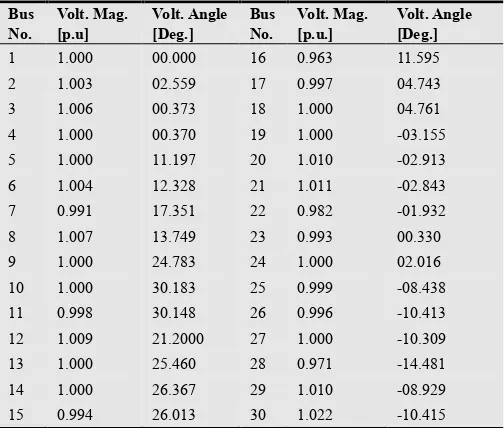
Table 6. Voltage magnitude and Voltage angle profiles: Tanzania network

Bus No.

Volt. Mag. [p.u]

Volt. Angle [Deg.]

Bus No.

Volt. Mag. [p.u.]

Volt. Angle [Deg.] 1 1.000 00.000 16 0.963 11.595 2 1.003 02.559 17 0.997 04.743 3 1.006 00.373 18 1.000 04.761 4 1.000 00.370 19 1.000 -03.155 5 1.000 11.197 20 1.010 -02.913 6 1.004 12.328 21 1.011 -02.843 7 0.991 17.351 22 0.982 -01.932 8 1.007 13.749 23 0.993 00.330 9 1.000 24.783 24 1.000 02.016 10 1.000 30.183 25 0.999 -08.438 11 0.998 30.148 26 0.996 -10.413 12 1.009 21.2000 27 1.000 -10.309 13 1.000 25.460 28 0.971 -14.481 14 1.000 26.367 29 1.010 -08.929 15 0.994 26.013 30 1.022 -10.415

Computational results are divided into A and B parts. Part A refers to results from IEEE 14 and IEEE 30 bus test systems. These results are presented to check the convergence characteristics of the developed MATLAB software. Part B presents result from the Tanzanian network model; computational result from this system are used to validate the one-line diagram model as well as validity of input data collected from Tanzania Electric Supply Company Limited (TANESCO). The computational results obtained after simulation are presented in both tabular and graphical form. Table 6 shows the corresponding voltage magnitude and voltage angle profile of the Tanzanian network. Table 7 presents a summary of load flow results of other IEEE standard bus test systems including the Tanzanian network. The aim of presenting this summary is to make comparison of/observe iteration counts for different IEEE bus test systems, maximum power mismatch; CPU time elapsed till convergence, total system loss, total MVAr system loss, and accuracy of the MATLAB software if it remains within pre-defined tolerance for all test systems. Figures 5 shows voltage magnitude profile and Figure 6 presents voltage angle profile of the Tanzania network.

Table 7. Summary of load flow results

Test System IEEE 14 IEEE 30 Tanzanian Network

Number of Lines 20 41 33 Transformer Tap setting FIXED FIXED FIXED Max. Power Mismatch 1.15E-008 1.20E-008 7.17E-007 No. of Iterations 10 9 4 Comp. Accuracy 0.0001 0.0001 0.0001 CPU time [Seconds] 2.270 3.191 3.088 Injected MVAr 00.00 00.00 00.00 Total MVAr Loss 31.618 23.611 -171.028 Total System Loss 13.483 17.730 28.041

VOLT AGE MAGNITUDE PROFILE-T ANZANIAN NET WORK

0.96 0.97 0.98 0.99 1 1.01 1.02 1.03

0 5 10 15 20 25 30 35

BUS NUMBER

V

O

L

T

A

G

E

M

A

G

N

IT

U

D

E

I

N

P

.U

.

VOLT AGE ANGLE PROFILE-T ANZANIAN NET WORK

-20 -10 0 10 20 30 40

0 10 20 30 40

BUS NUMBER

V

O

L

T

A

G

E

A

N

G

L

E

I

N

D

E

G

R

E

Figure 7b. Newton-Raphson Algorithm in Flowchart Format

7. Discussion

The following observations from simulation results can be made. The load flow solution for the Tanzanian network has

a maximum power mismatch of about 7.17x10-7; and

converged after 4 numbers of iterations. The total real and reactive power losses in the system during this particular scenario were 20.041 MW and -171.028 MVAr. The voltage magnitude and voltage angle profiles of the Tanzanian power network are within acceptable limits i.e. 0.95-1.10 per unit

for voltage magnitude and -350-+350 degree for voltage angle.

The power factor (pf) of the system is around 0.868 (+300

degree) which is the operating value required by TANESCO. It means that the selection of system components and modelling procedure was successful. Also, it means that the high voltage transmission system has the required nominal capacity to meet the current power demand.

8. Conclusion

This paper has presented an overview of the Tanzanian power network structure. Modelling procedure of critical system components for load flow analysis and their corresponding models have been developed and presented. An approximate model of the Tanzanian power network model is built from the developed models and used in load flow analysis. The load flow problem, which involves in determining voltage, and line flow in an electrical network is discussed and then formulated using Newton-Raphson algorithm. Algorithm formulation in form of flowchart and MATLAB software for simulation as well as results from simulation are developed and presented.

results can be used in other critical studies such as power system state estimation (PSSE), optimal power flow (OPF), security constrained optimal power flow (SCOPF) etc of the Tanzanian power network.

Acknowledgement

I would like to thank the Tanzania Electric Supply Company Limited (TANESCO) for its cooperation and readiness to supply most of the needed data and information to make this work possible. Their support is gratefully acknowledged.

References

[1] W.F. Tinney & C.E. Hart, Power flow solution by Newton’s method, IEEE Transactions on Power Apparatus and Systems, Vol. PAS-86, November 1967: 1447-1460

[2] A.O. Ekwue, & J.F. Macqueen, Comparison of Load Flow Solution Methods, Electric power System Research 22 (1991): 213-222

[3] L. Srivastava, S.C. Srivastava & L.P. Singh, Fast decoupled load flow methods in rectangular coordinates, Electrical Power and Energy Systems (1991): 160-166

[4] A.E. Guile & W.D. Paterson, Electrical Power Systems, Vol.2,( Pergamon Press, 2nd Edition, 1977)

[5] W.D. Stevenson Jr, Elements of Power System Analysis (McGraw-Hill, 4th Edition, 1982)

[6] B. Stott, Effective starting process for Newton-Raphson load flows, IEE Proceeding, 118, No. 8, August 1971: 983-987 [7] W.F. Tinney & W.L. Powel, Notes on Newton-Raphson

method for solution of AC power flow problem, IEEE Short course, Power System Planning, 1971

[8] B. Stott, Fast decoupled Newton Load flow, IEEE Transactions on Power Apparatus and Systems, Vol. PAS-91, October 1972: 1955-1959

[9] B. Stott & O. Alsac, Fast decoupled load flow, IEEE Transactions on Power Apparatus and Systems, Vol. PAS-83, 1974: 859-869

[10] http://www.tanesco.com/national.html [11] http://www.tanesco.com/generation.html [12] http://www.tanesco.com/trans.html

[13] S.S. Vadhera, Power System Analysis and Stability (Khanna Publishers, 1st Edition, 1981)

[14] J.J.Grainger & W.D. Stevenson Jr. Power System Analysis (McGraw-Hill, Inc. Singapore, 1994)

[15] J.A. Momoh, Electric Power System Application of Optimization (CRC Press, 2nd Edition, 2009)

[16] A. Monticelli, State Estimation in Electric Power Systems: A Generalized Approach. (Norwell, MA: Kluwer, 1999)

[17] J. Arrilaga, C.P.Arnold & B.J. Harker, Computer Modelling of Electrical Power Systems. (New York: Wiley, 1983)

[18] A.G. Exposito, Analisis y operacion de sistemas de energia Electrica-Madrid Spain (McGraw-Hill/Interamerican de Espana, 2002)

[19] H.Saadat, Power System Analysis. International Edition (McGraw-Hill, Singapore, 2nd Edition, 2004)

[20] A.R. Bergen & V.Vittal, Power System Analysis, International Edition (Pearson Prentice Hall, 2nd Edition, 2000)

[21] L. Powel, Power System Load Flow Analysis. (McGraw-Hill, New York, 2004)

[22] F.L. Alvarado, Solving Power flow Systems with MATLAB implementation of the Power System Application Data Dictionary, Proceedings of the 32nd Hawaii International Conference on System Science , Hawaii, USA , 1999, 1-7