Breast MRI segmentation for density estimation: Do different methods give the
1
same results and how much do differences matter?
2
Simon J. Doran,1,a) John H. Hipwell,2,b) Rachel Denholm,3 Bj¨orn Eiben,2 Marta 3
Busana,3 David J. Hawkes,2 Martin O. Leach,1 and Isabel dos Santos Silva3
4
1)Cancer Research UK Cancer Imaging Centre, Division of Radiotherapy
5
and Imaging, The Institute of Cancer Research, London, SM2 5NG, 6
UK. 7
2)Centre for Medical Image Computing (CMIC), Department of
8
Medical Physics and Bioengineering, UCL, London, WC1E 7JE, 9
UK. 10
3)Department of Non-Communicable Disease Epidemiology,
11
London School of Hygiene & Tropical Medicine, London, WC1E 7HT, 12
UK. 13
ABSTRACT
Purpose To compare two methods of automatic breast segmentation with each other and with manual segmentation in a large subject cohort. To discuss the factors involved in selecting the most appropriate algorithm for automatic segmentation and, in particular, to investigate the appropriateness of overlap measures (e.g., Dice and Jaccard coefficients) as the primary determinant in algorithm selection.
Methods Two methods of breast segmentation were applied to the task of calcu-lating MRI breast density in 200 subjects drawn from the Avon Longitudinal Study of Parents and Children, a large cohort study with an MRI component.
A semi-automated, bias-corrected, fuzzy C-means (BC-FCM) method was com-bined with morphological operations to segment the overall breast volume from in-phase Dixon images. The method makes use of novel, problem-specific insights. The resulting segmentation mask was then applied to the corresponding Dixon water and fat images, which were combined to give Dixon MRI density values. Contempora-neously acquired T1- and T2-weighted image datasets were analysed using a novel
and fully automated algorithm involving image filtering, landmark identification and explicit location of the pectoral muscle boundary. Within the region found, fat-water discrimination was performed using an Expectation Maximisation - Markov Random Field technique, yielding a second independent estimate of MRI density.
Results Images are presented for two individual women, demonstrating how the difficulty of the problem is highly subject-specific. Dice and Jaccard coefficients comparing the semiautomated BC-FCM method, operating on Dixon source data, with expert manual segmentation are presented. The corresponding results for the method based on T1- and T2-weighted data are slightly lower in the individual cases
shown, but scatter plots and inter-class correlations for the cohort as a whole show that both methods do an excellent job in segmenting and classifying breast tissue.
Conclusions Epidemiological results demonstrate that both methods of auto-mated segmentation are suitable for the chosen application and that it is important to consider a range of factors when choosing a segmentation algorithm, rather than focus narrowly on a single metric such as the Dice coefficient.
Keywords: breast cancer, MRI, mammographic density, ALSPAC, segmentation 16
a)Joint first author and corresponding author: [email protected]
I. INTRODUCTION 17
Mammographic density, a quantitative measure of radio-dense fibrogladular tissue in the 18
breast, is one of the strongest predictors of breast cancer risk. Women with more than 75% 19
density have a four-fold or higher risk of breast cancer compared to those with less than 5%1.
20
More intensive screening for women with high mammographic density has been proposed2
21
but remains controversial3.
22
However, in clinical practice, mammographic density, as assessed on x-ray mammograms, 23
is generally reported using only qualitative, radiologist-assessed categories, and agreement 24
between radiologists tends to be only moderate4. Quantitative analysis is hampered by the
25
fact that breast density is an inherently 3-D material property and therefore not well suited 26
to measurement using 2-D x-ray projections. Although subsequent risk assessment and epi-27
demiological analysis rarely use full 3-D information (normally preferring a single number, 28
i.e., the volume-averaged mean breast density), accurate derivation of such a statistic from 29
the 2-D X-ray data is problematic and subject to error. Automated tools such as Volpara 30
(VolparaSolutions, Wellington, NZ)5 and QUANTRA (Hologic Inc., USA) are gaining trac-31
tion in the mammography community, suggesting that mean breast density can be calculated 32
without inter-reader bias. However, such readings may be affected by errors in estimating 33
breast thickness6 and the relation between the values of breast density reported and those 34
obtained by other techniques remains to be elucidated7.
35
Increasingly, Magnetic Resonance Imaging (MRI) mammography is being used in clinical 36
and research settings to assess breast structure, because of its 3-D capabilities, its non-37
ionizing nature and the strong soft tissue contrast between fibroglandular (parenchymal) 38
and fatty tissue. In an MRI context, breast density refers to the percentage of breast tissue 39
volume that is deemed to be “parenchymal” and this is generally assumed to be the same as 40
volume fraction of tissue whose MR signal arises from free water molecules, as opposed to 41
fat (i.e., the “water fraction” or “percentage water”). Clearly, this is not an exact equivalent 42
of the mammographic x-ray density. Nevertheless, Thompson et al.8 demonstrate a clear
43
correlation between the two. 44
At present manual evaluation of MRI 3-D breast density is an arduous, observer-45
dependent, and time-consuming process. Therefore, full or partial automation of the 3-D 46
mal volume and breast fat volume, two separate image processing tasks are required. First, 48
the breast as a whole needs to be distinguished from the background and chest wall; and, 49
second, the parenchymal tissue within the breast needs to be distinguished from fat. 50
Several different MRI pulse sequences have previously been used to assess breast density, 51
but no definitive consensus has been reached about which is optimal. Few studies have 52
compared different sequences within the same subject population. Furthermore, whilst there 53
is a large body of prior literature (see Table I) describing different ways to achieve the two 54
segmentation tasks described above, no studies, to date, have compared different automated 55
methods with each other and with manual segmentation, for a sizeable subject population. 56
It is clear that many methods can produce “good” segmentation results. This study 57
poses the following question: Do the minor differences we see between segmentations when 58
we apply different algorithms on the same data actually matter for the uses to which the 59
segmentations are ultimately put? 60
This study compares two very different methods of breast-outline segmentation: (i) an 61
established37 bias-corrected fuzzy C-means (BC-FCM) clustering technique based on a
cost-62
function; and (ii) a new heuristic approach based on thresholding, landmark identification 63
and direct analysis of image features. The results of this part of the study will be measures of 64
overall breast volume from each method and volume similarity measures (Dice and Jaccard 65
coefficients). 66
With the breast outline obtained, the second part of the study compares two methods 67
of fat-water discrimination, again based on different principles: (i) The Dixon approach38 68
uses scans acquired with an MRI technique that returns separate “fat” and “water” images. 69
In principle, these allow us to obtain a fat and water fraction for every voxel, accounting 70
for partial volume effects. However, Dixon sequences are not currently part of the routine 71
acquisition protocol for clinical MRI examinations39. (ii) Our second method uses an analysis
72
of the intensity histograms of the two different tissue classes in fat-suppressed T1-weighted
73
(T1w) and T2-weighted (T2w) images. Such images are routinely acquired in diagnostic
74
scanning and this method thus has the potential advantage of wider applicability if the two 75
methods are shown to be concordant. Note that there is no means of obtaining ground truth 76
data and, given that we are dealing with a healthy subject cohort, no possibility of obtaining 77
x-ray data for comparison. 78
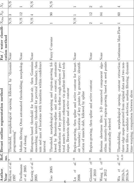
TABLE I: Summary of journal papers describing methods to segment pectoral muscle and internal fibro-glandular tissue from MR images. NOB refers to the number of observers who provided the gold standard manual segmentation. ND indicates the number of MR data sets the method was validated with and NS the number of MRI scanners. N/A = not
applicable; N/S = not specified
A comprehensive epidemiological analysis of the relationship between breast composition 80
and seven other physical, historical and lifestyle variables has been carried out for this cohort. 81
Whilst the full report is beyond the scope of this study, we summarise the results and use 82
them to discuss quantitatively the impact of differences between the various assessment 83
methods on conducting reliable clinico-epidemiological studies. 84
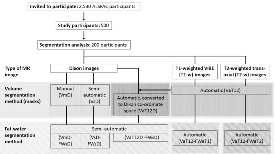
FIG. 1: Flow diagram of the overall data processing chain and nomenclature for the various segmentation methods. Some of these have the potential to operate on different source data and we can also combine the methods in different ways to achieve an overall result. We thus assign each step three codes: segmentation purpose (V = breast volume, FW = fat-water); degree of automation (m = manual, s = semi-automatic, a = fully automatic); and source data (D = Dixon; T1 = T1-weighted,
T2 = T2-weighted, T12 = uses both T1- and T2-weighted data). Thus, a
breast-volume measurement using semi-automatic segmentation on original Dixon data would be represented as VsD. Fat-water segmentations require both source data and a previously-generated volume mask, so are represented by the combination of two codes. For instance, fat-water statistics calculated semi-automatically from Dixon source data and using a mask generated automatically from T1w and T2w data would be described by VaT12-FWsD. We note one additional case, in which the volume mask VaT12 is re-sampled to give a result in the same coordinate space
II. METHODS 85
A. Data 86
1. Study Population 87
This work forms part of an investigation into breast composition at young ages, nested 88
within the Avon Longitudinal Study of Parents and Children (ALSPAC). ALSPAC originally 89
recruited 14,541 pregnant women resident in Avon, UK with expected dates of delivery 1st 90
April 1991 to 31st December 1992, as described by Boydet al.in a cohort profile paper40. For 91
this sub-study, Caucasian nulliparous women were invited to attend an MRI examination at 92
the University of Bristol Clinical Research and Imaging Centre (CRIC) between June 2011 93
and November 2014. Women were restricted to those from a singleton birth, who had never 94
been diagnosed with a hormone-related disease and had regularly participated in follow-up 95
surveys, including completing the age 20y questionnaire (2010-2011). Of the 2530 invited, 96
500 (19.8%) eligible women attended. 97
The ALSPAC Law and Ethics Committee and the Local Research Ethics Committees 98
gave ethical approval for the study. The study website contains details of all the data that 99
are available through a fully searchable data dictionary41.
100
2. MR Imaging 101
Participants underwent a breast MRI scan using a 3T Siemens Skyra MR system with 102
a breast coil that surrounds both breasts of a prone patient. Three sets of bilateral images 103
were acquired: 104
• multislice, sagittal Dixon38 images (in-phase, out-of-phase, water and fat), acquired
105
using a turbo spin-echo sequence with nominal in-plane resolution of (0.742 × 0.742) 106
mm2, nominal slice thickness 7 mm and interslice spacing 7.7 mm; 107
• T1-weighted 3D images, acquired using a VIBE sequence with fat saturation and 108
a nominal resolution of (0.759 × 0.759 × 0.900) mm3, as routinely used in clinical
109
dynamic contrast-enhanced MRI protocols for the breast; 110
nominal in-plane resolution of (0.848 × 0.848) mm2, and both slice thickness and
112
spacing between slices 4 mm; 113
3. Manual Reference Segmentation 114
To assess breast volume, a manual segmentation protocol (as described in the Supplemen-115
tary Information) was developed and used by three readers (RD, MB and ISS) independently 116
to outline the breast from surrounding tissues in the Dixon images, using ITK-SNAP (ver-117
sion 3.0.0). All subjects had a manual segmentation of all breast slices performed by at least 118
one reader. The datasets of 16 representative subjects were manually segmented twice by 119
all three readers to assess between- and within-observer variation. In cases where more than 120
one manual segmentation is performed, the VmD and VmD-FWsD results quoted below 121
represent the median values taken for the multiple manual readings. 122
4. Training and Validation Data Sets 123
A training set of 100 randomly selected subjects was used to make initial comparisons 124
across MR images and segmentation methods, and for the manual readings, between- and 125
within-observer variation. The training data were used to assess the common reasons for 126
segmentation failure and to improve the algorithms. At the end of the testing phase, the 127
algorithm code was “frozen” and final comparisons of the segmentation methods were com-128
pleted on a second set of images from a further 100 participants. Except where stated other-129
wise, all the summary statistical results presented here come from this second, “validation” 130
cohort. For further details concerning statistical methods, please see the Supplementary 131
Information. 132
B. Breast Outline Segmentation 133
1. Semi-automated, bias-corrected fuzzy C-means (BC-FCM) 134
A fuzzy C-means (FCM) algorithm was applied to the Dixon in-phase images. It has 135
the advantage that it can be modified to carry out a simultaneous intensity inhomogeneity 136
than a prefiltering operation42. The algorithms in this section were implemented using IDL
138
(Harris Geospatial Systems, Melbourne, FL, USA) and run on a standard desktop computer. 139
The BC-FCM variant we implemented is described in37. Formally, the algorithm does not 140
require a training dataset and so is an unsupervised clustering algorithm. However, in prac-141
tice, some experience with the types of data involved can improve the results dramatically. 142
Except for the local smoothness criterion (introduced by cost function γ in ref.37 — see this 143
publication for all other related notation), BC-FCM per se does not use any spatial infor-144
mation. Nevertheless, a “good” segmentation involves a number of problem-specific insights 145
and the basic BC-FCM method above was enhanced by additional heuristic algorithms in 146
the spatial domain, based on the results obtained with the training data. 147
a. Initial parameters and iteration threshold After some experimentation,β(r) was set 148
to 0.1 for all spatial locations andto 0.01. The two initial class centroidscf were calculated 149
by taking the mean of the slice being processed and adding a lower and an upper offset. 150
These two offsets are adjustable parameters under user control. For many subjects — see the 151
Results section for an example —, a single set of defaults performed extremely well. However, 152
for a small subset of “difficult” cases — second example in Results —, user interaction was 153
needed to try various combinations. As implemented here, on a standard desktop computer, 154
running non-optimised software, it took around 2 mins. to run the segmentation algorithm 155
on each 3-D dataset. Thus, this “trial and error” step was the most frustrating feature 156
of the BC-FCM method in practice. Numerous coding and hardware improvements (e.g., 157
parallelisation) could be made to the prototype to improve the user experience, potentially 158
allowing these adjustable parameters to be altered by simple slider controls with immediate 159
feedback. 160
We observed an improvement in performance by allowing the algorithm to perform sep-161
arate BC-FCM classifications for segmenting the posterior of the breast from the chest wall 162
and segmenting the anterior portion from air, then merging the two volumes. Furthermore, 163
it was noted that the optimal offsets providing the initial class centroids were often differ-164
ent for these two segmentation problems. Thus, each dataset is split into two portions in 165
an anterior-posterior (AP) direction and the BC-FCM algorithm applied twice per image 166
slice. Given that the size of breasts varies, the position of the AP-split is also different for 167
different datasets and this is handled automatically by having two passes through the entire 168
b. Morphological operations The breast outlining task requires a definite boundary to 170
be drawn. Thus, it is not necessary to use the full membership function output of the 171
BC-FCM routine, and we arrange for the clustering to produce a binary image. This may 172
include some misclassified regions outside the breast and some “holes” inside the breast. To 173
remove the unwanted regions, 2D hole-filling followed by a 4-neighbourhood connectivity 174
search and object labelling is performed. The largest non-background object in each slice is 175
identified as the breast region and other smaller objects are removed from the binary image. 176
This exercise is repeated for all slices and these are then merged to form an approximate 177
breast volume. 178
Within this approximate breast volume, there may be some non-breast tissue segmented 179
for cases in which fatty breast tissue is connected to the chest and liver; and there may also 180
be some unsegmented breast tissue left for cases in which dense breast tissue is connected to 181
the chest wall muscles. To reduce these over- and under-segmentations, 3D morphological 182
image opening is performed, followed by closing using two cylindrical structuring elements 183
having the same radius of 3 voxels but different heights of 3 voxels and 25 voxels in the axial 184
direction. These parameters were found by experimentation during our previous study37.
185
c. Lateral cutoffs The preceding steps in the process do an excellent job in segmenting 186
the anterior and posterior margins of the breast. However, there is no consensus in the 187
literature as to “where the breast stops” in the right-left and superior-inferior directions. 188
The extent of the breast is not directly delineated by any change in MRI contrast and the 189
required boundary may, indeed, be specific to the application of the imaging (e.g., when 190
comparing the MRI segmentation with the breast region compressed within the paddles 191
of a mammography system, the axilla region may be excluded entirely). Thus, based on 192
the consensus protocol (Appendix??) reached by the three experienced readers, a heuristic 193
algorithm was developed, as described below. This additional truncation is derived entirely 194
from geometric considerations and boundaries are drawn without regard to image intensity, 195
which is in many cases the same on either side of the boundary. 196
Each breast is processed in turn. The stack of sagittal images segmented using BC-197
FCM forms a pseudo 3-D dataset. From this dataset the transverse plane containing the 198
largest breast area is passed to a simple algorithm that extracts the air-breast interface as 199
a 1-D “breast profile”. (This geometry is illustrated as Figure S2 of the Supplementary 200
right direction. Working outwards from this midpoint, we find the first position at which 202
the absolute value of the gradient (approximated by the finite difference between adjacent 203
voxels) of the breast profile rises above a threshold value, determined by experimentation. 204
This indicates a change in angle of the skin surface from flat regions between and outside 205
the breasts, to the side contour of the breast. A mask is applied to exclude all sagittal slices 206
in the original dataset on either side of these changes in angle. (Typically, the “raw” output 207
of the BC-FCM algorithm would include these.) Finally, a similar profile is generated for 208
the superior-inferior direction and the upper and lower bounds of the breast are determined 209
in each sagittal plane of the original data. 210
2. Fully-automated, using T1w and T2w Images 211
a. Pre-Processing Processing (Bias-Field Correction) A slowly varying bias-field, 212
caused by inhomogeneities in the magnetic field during the MR acquisition, is a com-213
mon artefact of MR images. To correct this for the T1w and T2w images, we apply the 214
“N4ITK” nonparametric non-uniform intensity normalization method43. This is a
refine-215
ment of the popular N3 algorithm which adopts a fast, robust B-spline fitting algorithm 216
and a hierarchical, multi-scale, optimisation scheme (figures 2a and 2b). 217
b. Breast Mask Segmentation This novel, heuristic method, implemented using the 218
Insight Toolkit44, computes a whole breast mask using both the T1w and T2w images.
219
In developing this automated approach, emphasis has been placed on limiting the number 220
of empirically derived parameters and relying instead on detecting statistical or functional 221
extrema. In this way we aim to make the method as widely applicable to variations in 222
subjects and images as possble. The method comprises a number of distinct processing 223
steps as follows. 224
1. The T2w image is resampled to match the resolution of the T1w image. 225
2. A grey-scale closing operation along each of the orthogonal axes, x, y and z, is per-226
formed on the T2w image, to eliminate voids from the subsequent foreground segmen-227
tation. In this operation each voxel’s intensity, IT2w, at index (i, j, k) is replaced by
228
IcT2w(i, j, k) according to:
IcT2w(i, j, k) = min
"
min
max
0≤i1≤iIT2w(i1, j, k),i<imax2<Ni
IT2w(i2, j, k)
,
min
max
0≤j1≤j
IT2w(i, j1, k), max j<j2<Nj
IT2w(i, j2, k)
,
min
max
0≤k1≤k
IT2w(i, j, k1), max k<k2<Nk
IT2w(i, j, k2)
#
(1)
where Ni,Nj, Nk are the number of voxels along each axis. 230
3. The T1w image is rescaled to match the intensity range of the closed T2w image and 231
the maximum of these two images, IMaxT1wT2w, computed.
232
4. The foreground (i.e. the subject) is segmented from the background by thresholding, 233
IMaxT1wT2w. The threshold, tbg, is computed via:
234
tbg = arg max I
[Fdark(I) (FCDT(I)−Fvar(I))] (2)
according to the following functional criteria: 235
• The background is assumed dark therefore the threshold should be close to zero: 236
Fdark(I) = 1−
I
max(I) (3)
• The frequency of voxel intensities in the background is higher than the foreground 237
i.e. the background intensities form a distinctive peak in the image histogram, 238
P(I), which is captured by a sharp rise in the cumulative intensity distribution 239
function: 240
FCDT(I) =
PI
j=0P(j)
Pmax(I)
k=0 P(k)
(4)
• The background has a lower intensity variance than the foreground: 241
Fvar(I) =
PI
j=0P(j)(j−µ)2
Pmax(I)
k=0 P(k)(k−µ)2
(5)
The resulting foreground mask image is denoted Ifg — see Figure 2(d).
(a) Original MRI T2w acquisition.
(b) Bias-field corrected image.
(c) Closed image. (d) Foreground mask.
FIG. 2: Orthogonal slices through (a) a T2 weighted MRI and (b) the corresponding image after bias-field correction, with arrows indicating regions that are particularly im-proved by the processing. The “closed” T2w image is shown in (c) and foreground maskIfg in (d). In each image the top-left quadrant is the axial slice, the top-right
is sagittal and the bottom-left is coronal.
5. Landmark identification. The most anterior voxels in the foreground mask, Ifg, on
243
the left and right sides of the volume, are identified and assumed to be approximately 244
coincident with the nipple locations. If multiple voxels are found then the center of 245
mass of the cluster is computed. The mid-sternum is computed as the most anterior 246
voxel of the foreground mask, equidistant from the nipple landmarks in the coronal 247
plane. 248
6. Pectoral muscle boundary extraction. Various methods have been presented in the 249
literature to segment breast MRI volumes and the pectoral muscle (Table I). These 250
include semi-automated methods requiring user interaction31,33,36, 2D mid-slice tem-251
plate registration36, statistical shape models25 and atlas-based methods16,18–20,24,45.
(a) Detected “dark line” structures.
(b) Pectoral mask. (c) Extrapolated B-Spline
surface mask.
FIG. 3: The anterior pectoral muscle surface is detected using the Oriented Basic Image Feature “dark line” class. Subplot (a) shows these features detected at four ori-entations (OBIF15 to OBIF18). Region-growing the “brown” medial-lateral class,
OBIF15, closely delineates this anterior boundary immediately posterior to the
ster-num (b). The anterior surface of this mask is extrapolated using a B-Spline fit to the lateral boundaries of the volume (c).
(a) Right breast outline. (b) Left breast outline.
(c) Surface rendering.
FIG. 4: Breast region mask created by removing the pectoral surface mask (figure 3c) from the foreground mask (figure 2d). Two views of the mask are shown, superimposed on the original MR image and centered on the right (a) and left (b) breasts. The
A number of methods have been developed to segment explicitly the pectoral mus-253
cle. These include a B-spline fit to the intensity gradient of the pectoral boundary33,
254
anisotropic diffusion and Canny edge detection17 and Hessian matrix planar shape
255
filtering15,46. Atlas-based methods have been shown to perform well but are compu-256
tationally intensive47 and require significant initial investment of time to develop a
257
library of atlases. 258
We have developed a method to detect explicitly the anterior pectoral muscle boundary 259
in individual MR volumes. Our approach has similarities to the Hessian processing 260
of Wang et al.15,46, in that it employs Gaussian derivatives to detect regions in the
261
image with a planar profile. However rather than computing a ratio of the eigenvalues 262
of the Hessian matrix and thresholding the result, we obtain a direct classification of 263
linear structures, immediately posterior to the sternum, using Oriented Basic Image 264
Features (OBIFs, Figure 3). 265
The concept of Basic Image Features (BIFs) was developed by Griffin48. The technique
266
classifies pixels in a 2D image into one of seven classes according to the local zero-, first-267
or second-order structure. This structure is computed using a bank of six derivative 268
of Gaussian filters (L00, L10, L01, L20, L11 and L02) which calculate the nth (where
269
n=0,1,2) order derivatives of the image in x and y (S00, S10, S01, S20, S11 and S02).
270
By combining the outputs of these filters, any given pixel can be classified according 271
to the largest component of vector BIF: 272
BIF =
(
flat
S00,
slope−like
2
q
S2
10+S012 , maximum
λ ,
minimum
−λ ,
light line
λ+γ
√
2 ,
dark line
λ−γ
√
2 ,
saddle
γ
)
given 273
λ=σ2(S20+S02)
2 (7)
γ =σ2
q
(S20+S02)2+ 4S112 (8)
(9)
In addition, slopes, light lines, dark lines and saddles can be characterised according to 274
their orientation (OBIFs). We quantise this orientation into four, 45 degree quadrants 275
which produces eight slope sub-classes (OBIF1 to OBIF8), and four sub-classes for
276
each of light lines (OBIF11 to OBIF14), dark lines (OBIF15 to OBIF18) and saddles
277
(OBIF19 to OBIF22).
278
By region-growing the medial-lateral, OBIF15 dark line features detected in each axial
279
image slice, in 3-D, from seed positions immediately posterior to the mid-sternum, 280
we obtain a binary segmentation of the anterior pectoral muscle surface. The BIF 281
processing was performed at a single scale using a Gaussian kernel with standard 282
deviation 5 mm. A smooth B-spline surface is then fitted to the anterior voxels of 283
the resulting mask44 to extrapolate the muscle surface to the lateral boundaries of the
284
image volume (figure 3c). 285
7. Finally we generate a 2D coronal mask, ICNL, to crop non-breast tissue from the
286
whole breast mask. ICNL is computed from a coronal skin elevation map, Iskin2D, 287
which contains the distance of each anterior skin voxel in the foreground mask, Ifg,
288
from the most posterior boundary of the MR volume. The coronal profile of each 289
breast is obtained by thresholdingIskin2D at 290
h= (4hms+hLn+hRn
6 (10)
wherehms is the anterior elevation of the mid-sternum landmark, andhLn and hRn are
291
the left and right nipple anterior elevations respectively. The roughly circular profile 292
obtained for each breast is then dilated by 10mm and the mask squared off, to create 293
C. Fat-Water Discrimination 295
1. Semi-automated calculation of percentage breast density, based on Dixon 296
Images 297
In principle, the output from a Dixon pulse sequence is a set of images reflecting water 298
content Iw(r), which we identify with the parenchymal component of the breast, and an 299
equivalent set If(r) reflecting fat content. Ideally, these images would be quantitative and 300
allow the direct calculation of the water and fat fractionsφw(r) andφf(r) via the equation49 301
φw = Iw Iw+If
and φf = If Iw+If
(11) In practice, there are a number of complicating factors:
302
• Parenchymal tissue and fat have different relaxation properties and, since the acqui-303
sitions are not generally designed to be proton density weighted, this means that the 304
relative intensities of equal fractions of fat and water are different. 305
• The B1 field of the probe is not uniform across the whole breast and this leads to a
306
spatially-dependent efficacy of the fat-water separation. 307
• In practice, the fat tissue does not have a single proton resonance. 308
• Different manufacturers have different proprietary image reconstruction methods and 309
these may influence the quantitative results. 310
Our solution to (at least) the first of these problems is to proceed as follows: 311
(a) Identify a small region in the water image that is expected to be entirely composed 312
of parenchymal tissue. The region should be in a part of the image that is free from 313
intensity artefacts caused by proximity to the RF coil (i.e., the data should come from 314
a homogenous region of B1).
315
(b) In the fat image, identify similarly a second region entirely composed of fat. 316
(c) Calculate the ratio of the average voxel values in each of the two regions: 317
r = 1 Nw
X
i∈ROIw
Iw(ri)
1 Nf
X
j∈ROIf
whereNw and Nf are the numbers of voxels in the selected regions-of-interest ROIw and 318
ROIf respectively. 319
(d) Replace the value If in Eq. (11) with rIf. 320
This procedure potentially improves the accuracy of the water-fraction calculation but at 321
the cost of introducing an interactive step into the density estimation process. We have not 322
tested in a systematic fashion the influence that the size and shape of the region-of-interest 323
selection have on the process, in part because we have no ground truth values. A further 324
issue with this technique is that in the limiting cases of extremely dense or extremely fatty 325
tissues, it may not be possible to find appropriately “pure” regions of both types. 326
2. Fully-automated, using T1w and T2w Images 327
Fuzzy c-means (FCM) clustering has been evaluated by a number of studies to classify 328
the internal structure of the breast into fat and fibro-glandular tissue classes16,18,29,31,33–35,50 329
Table I). Songet al.50adopt a Gaussian kernel FCM, whilst Sathya34use a quadratic kernel
330
FCM to train a support vector machine (SVM). In29, Wang et al. use a multi-parametric
331
hierarchical SVM classification approach to segment the internal breast and found this to be 332
superior to both a conventional SVM28and FCM segmentation. T1W, T2W, proton density
333
and three point Dixon (water and fat) images were all incorporated. Klifaet al.31compared 334
the resulting volumentric MRI density measurement of their method with mammography 335
but found only modest correlation (R2 = 0.67).
336
In20 a probabilistic atlas approach was proposed. This requires a sizeable number of 337
pre-labelled atlases to be created, considerable computation to register them and assumes 338
correspondence between fibro-glandular structures across the population. To address the 339
latter a Markov Random Field (MRF) was introduced to spatially regularise the classification 340
of each voxel according to that of its neighbours. Similarly Wuet al.16use the registered atlas
341
as a pixel-wise fibroglandular likelihood prior for a multivariate Gaussian mixture model and 342
demonstrate superior performance when compared to FCM using a manual thresholding 343
approach as the gold standard. In a later publication19, the same authors investigate a
344
continuous max-flow (CMF) algorithm to generate a voxel-wise likelihood map using the 345
atlas initialisation than without, but that FCM is superior to the CMF approach without 347
the atlas. 348
Mixture models have also been proposed by Yang et al.32who implement a method using 349
Kalman filter-based linear mixing. They demonstrate it out-performs a c-means method but 350
evaluation using real MR data was limited. 351
Our segmentation of the T1 and T2 MRI data into fat and glandular tissue is a mod-352
ification of that proposed by Van Leemput et al.51 in which an intensity model and
spa-353
tial regularization scheme are optimized using a Maximum Likelihood formulation of the 354
Expectation-Maximisation (EM) algorithm. The EM algorithm iteratively updates the 355
Gaussian probability distributions used to estimate the intensity histograms of each tis-356
sue class (fat and non-fat) via a Maximum Likelihood formulation. In order to improve 357
classification of voxels in which the partial volume of fat and glandular tissues is a signif-358
icant factor, a Markov Random Field (MRF) regularization scheme is employed to ensure 359
spatial consistency. The MRF modifies the probability of a particular voxel being assigned 360
to either the fat or glandular classes (or a proportion of either) according to the current clas-361
sification of neighbouring voxels. In this way isolated regions of glandular tissue in very fatty 362
regions, for instance, are penalized in favour of a more realistic and anatomically correct 363
arrangement of the classes. 364
D. Epidemiology 365
Appropriate linear and logistic regression models were used to examine associations of 366
average total breast, fat and water volumes, and percent water, as measured using different 367
MR images and segmentation methods, with selected established and potential mammo-368
graphic density correlates. Breast measures were log-transformed and the exponentiated 369
estimated regression parameters represent the relative change (RC) in breast measure with 370
a unit increase, or category change, in the exposure of interest (with 95% confidence intervals 371
(95% CI) calculated by exponentiating the original 95% CIs). Age at menarche (months), 372
height (cm) and BMI (height (cm)/ weight (kg)2) at MR were treated as continuous
vari-373
ables and centred at the mean. Current hormone contraceptive use, cigarette smoking and 374
alcohol drinking were treated as binary (yes/no) variables. Mothers mammographic den-375
and clinically measured or self-reported maternal BMI (median 3 years (inter-quartile range 377
(IQR) = 1.5 years) prior to mammography)) were used as continuous measures and centred 378
at the mean. Variables were included as potential determinants of breast measures, or as 379
confounding factors, where appropriate. 380
Data analysis was conducted with STATA statistical software, Version 14. 381
III. RESULTS 382
A. Breast Outline Segmentation 383
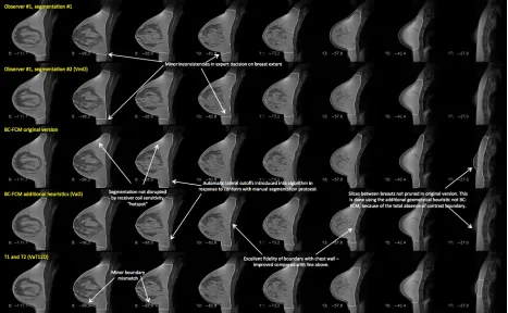
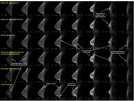
FIG. 5: : Example of a case where both of the algorithms examined in this work performed well. Features of interest in the various different segmentations are annotated.
Note that this image is provided with high resolution and can be zoomed significantly to reveal additional detail.
Figure 5 shows an example of the two methods applied to a dataset containing medium-384
sized breasts, with a moderate parenchymal content. There is a border of fat around the 385
parenchyma, which, at the posterior of the breast, leads to excellent contrast at the bound-386
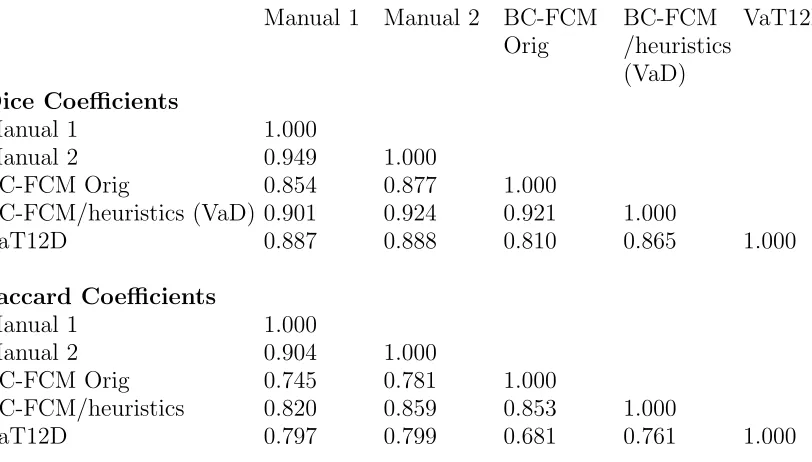
TABLE II: : Dice and Jaccard coefficients for the “easy” segmentation problem of Fig. 5. Note that the BC-FCM/heuristics (VaD) represents the fully automated version, running
with default parameters. Manual 1 Manual 2 BC-FCM
Orig
BC-FCM /heuristics (VaD)
VaT12D
Dice Coefficients
Manual 1 1.000
Manual 2 0.949 1.000
BC-FCM Orig 0.854 0.877 1.000
BC-FCM/heuristics (VaD) 0.901 0.924 0.921 1.000
VaT12D 0.887 0.888 0.810 0.865 1.000
Jaccard Coefficients
Manual 1 1.000
Manual 2 0.904 1.000
BC-FCM Orig 0.745 0.781 1.000
BC-FCM/heuristics 0.820 0.859 0.853 1.000
VaT12D 0.797 0.799 0.681 0.761 1.000
shown for two separate manual segmentations by the same experienced observer; for the 388
BC-FCM method from ref.37; the BC-FCM method with additional heuristics and default 389
parameters, as described above; and the new method based on T1 and T2 images (VaT12). 390
It will be seen that the segmentation performance is excellent, with only minor difference 391
between the methods. Note how implementation of guidelines developed during the manual 392
segmentation process supplements the BC-FCM approach in order to cut off the segmenta-393
tion in both the left-right and superior-inferior directions, where there are no corresponding 394
intensity boundaries seen in the image data themselves. 395
Table II shows the Dice and Jaccard coefficients for the four sets of segmentations illus-396
trated in Figure 5, confirming the excellent performance of all the algorithms. 397
By contrast, Figure 6 illustrates a case where all assessment methods have far more 398
difficulty in providing a correct segmentation. Smaller breasts tend to be more problematic 399
to segment, as a higher fraction of the segmentation involves partial-volume effects. Highly 400
parenchymal breasts have very low (sometimes no) contrast between the parenchyma and 401
pectoral muscles of the chest wall, and the intensity-based BC-FCM algorithm has particular 402
difficulties in this regard. Many slices require a high degree of anatomical knowledge to 403
perform the segmentation. Consider the two versions of the BC-FCM results presented. 404
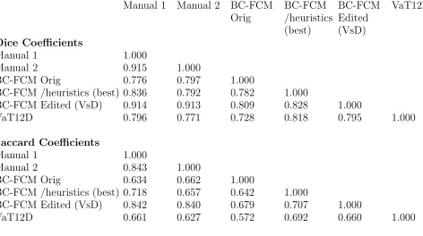
TABLE III: : Dice and Jaccard coefficients for the difficult segmentation problem of Fig. 6 Manual 1 Manual 2 BC-FCM
Orig
BC-FCM /heuristics (best)
BC-FCM Edited (VsD)
VaT12D
Dice Coefficients
Manual 1 1.000
Manual 2 0.915 1.000
BC-FCM Orig 0.776 0.797 1.000
BC-FCM /heuristics (best) 0.836 0.792 0.782 1.000
BC-FCM Edited (VsD) 0.914 0.913 0.809 0.828 1.000
VaT12D 0.796 0.771 0.728 0.818 0.795 1.000
Jaccard Coefficients
Manual 1 1.000
Manual 2 0.843 1.000
BC-FCM Orig 0.634 0.662 1.000
BC-FCM /heuristics (best) 0.718 0.657 0.642 1.000
BC-FCM Edited (VsD) 0.842 0.840 0.679 0.707 1.000
VaT12D 0.661 0.627 0.572 0.692 0.660 1.000
11 and part of the chest wall is included in the parenchymal breast region. By contrast, with 406
the “best” set of parameters (as found by repeating the algorithm and manually adjusting 407
them), the lower row shows that the problem in slice 11 is corrected, with good matching of 408
the pectoral muscle contour, but only at the cost of introducing an under-segmentation in 409
slice 8, and, worse, losing the segmented breast region entirely in slice 6. In practice, where 410
such problems occurred, it was necessary to edit the final segmentations manually. (Note on 411
terminology: As shown in Fig. 6, the “BC-FCM/heuristics (VaD)” method cannot reliably 412
be run for the whole cohort using only default parameters and so we must describe the 413
technique as semi- rather than fully-automated. Even for cases where no manual editing or 414
parameter adjustment need to be performed, human inspection is still required to confirm 415
this. All subsequent cohort statistics will therefore use the nomenclature VsD to reflect 416
this.) 417
We have run a similar analysis on all 16 cases for which we have duplicate manual 418
segmentations by all three observers. The detailed results are shown in the Supplementary 419
Information. 420
A second method of examining the relation between the volume segmentation results is 421
FIG. 6: : Example of a case where automatic segmentation is difficult. The rows represent the results of different segmentations and, for compactness, an informative subset of slices has been chosen to illustrate important features of the problem. Note that this image is provided with high resolution and can be zoomed significantly to reveal additional detail.
scatter plots of Figures 7(a)–(c), thex- and y-coordinates of each point represent the mean, 423
for a single subject, of the left and right breast volumes evaluated, respectively, by the two 424
methods under consideration. Figure 7(a) compares VsD, the semi-automated BC-FCM 425
method using Dixon image input, with the “gold-standard” median manual segmentation, 426
VmD, measured on the same Dixon dataset. Figure 7(b) gives results for the VaT12 method, 427
which operates on the T1w and T2w datasets and evaluates the breast volume in the coor-428
dinate space of the T1w dataset. Finally, Figure 7(c) looks at the effect of resampling the 429
map generated by the algorithm in (b) with the spatial resolution and frame of reference of 430
the Dixon data, which we term VaT12D. In each case, the line of identity is shown and Ta-431
ble IV reports the corresponding inter-class correlations (ICC), representing the proportion 432
(a) (b)
(c)
FIG. 7: Scatter plots of mean left and right breast volumes in cm3 for the different
methods in comparison to manual segmentation: (a) volume from semiautomatic segmentation of Dixon images (VsD) vs volume from manual segmentation (VmD); (b)
volume via automated segmentation from T1- and T2-weighted images transformed to
Dixon reference frame (VaT12FD) vs manual (VmD); (c) volume obtained from T1- and
T2-weighted images in native 3-D reference frame (VaT12).
TABLE IV: : Inter-class correlations for total breast volume segmentations.
VmD VsD VaT12D VaT12
VmD 1.000
VsD 0.990 1.000
VaT12D 0.974 0.977 1.000
TABLE V: : Inter-class correlations for total water volume segmentations. VmD-FWsD VsD-FWsD
VaT12D-FWsD
VaT12-FWaT1
VaT12-FWaT2 VmD-FWsD 1.000
VsD-FWsD 0.995 1.000
VaT12D-FWsD 0.992 0.993 1.000
VaT12-FWaT1 0.920 0.921 0.924 1.000
VaT12-FWaT2 0.948 0.949 0.962 0.899 1.000
B. Fat-Water Segmentation 434
Figures 8 and 9 present the results of the fat and water segmentation in the same format 435
as for the total breast volume. In this case, however, a further option is available. Although 436
the breast outline segmentation VaT12 requires both the T1w and T2w data, once this 437
mask is available, it is possible to obtain two separate fat-water segmentations one using 438
just the T1w and one using just the T2w data. These are denoted VaT12-FWaT1 and 439
VaT12-FWaT2 respectively. 440
The inter-class correlation (ICC) for total water volume, representing the proportion of 441
variance across participants shared between the different ascertainment methods, are given 442
in table V. 443
C. Epidemiological Results 444
A diagrammatic summary of the results of the epidemiological analysis is presented in 445
Figure 10 and further details of the work are reported as supplementary information. 446
Associations with both breast volume and breast water fraction were found for current 447
body mass index (BMI). For a 1 kg m−2 increase in BMI, a relative change in breast volume 448
of 1.13[1.10, 1.16] was observed for the cohort for both the VmD and VsD methods and 449
the corresponding result for the VaT12 family of methods was 1.15[1.12, 1.18], where the 450
figures in square brackets are the 95% confidence intervals. A smaller, but still important, 451
decrease in breast water fraction was seen, and the corresponding statistics are VmD-FWsD, 452
VsD-FWsD 0.96[0.95, 0.97], VaT12D-FWsD 0.95[0.94, 0.97], VaT12-FWaT1 0.97[096, 098], 453
VaT12-FWT2 0.95[0.94, 0.96]. 454
a 1 cm increase in height, the analysis methods gave the following relative increases in 456
breast volume: VmD 1.05[0.98, 1.11], VsD 1.04[0.98,1.11], VaT12D-FWsD was 1.05[0.97, 457
1.12], VaT12-FWaT1 1.05[095, 1.03], VaT12-FWT2 1.05[0.95, 1.13]. However, height was 458
not associated with breast water fraction. 459
No associations were found with any of: age of menarche, use of oral contraception, 460
smoking, alcohol intake or maternal mammographic density. 461
From the similarity of all these statistics, we conclude that the exact details of the seg-462
mentation methods are not significant at the level of this cohort analysis. 463
IV. DISCUSSION
464
Our results show that, as in many segmentation problems, the degree of success of the au-465
tomated algorithms varies significantly between subjects. Figure 5 and Table II demonstrate 466
excellent performance by all of the algorithms, whereas the degree of correspondence with 467
the expert manual segmentation is considerably poorer in Figure 6 and Table III. However, 468
it should be noted that even the expert human observer is less able to provide a good repeat 469
segmentation. 470
The ICCs for total breast volume in Table IV demonstrate good agreement between 471
all methods, but interestingly, slightly closer agreement between VaT12 and the two Dixon-472
based methods (VmD or VsD) than between VaT12D and the Dixon methods. As described 473
above, VaT12D is created by simply resampling VaT12 in the Dixon coordinate space, which 474
has a coarser slice thickness, using appropriate blurring and nearest neighbour interpolation. 475
Although movement between the Dixon and T1w or T2w scans could explain this disparity, 476
registering the volumes did not improve the results. The resampling process appears to 477
amplify the difference between VaT12 and VmD or VsD, but we have not analysed this 478
further, given that it is a relatively small effect. 479
It would, of course, be interesting to compare the output of the VaT1T2 method di-480
rectly with manual segmentation of the high-resolution T1w dataset in its native refer-481
ence frame, without the need to down-sample. However, the workload involved in creating 482
high-resolution manual segmentations is prohibitive. In the Supplementary Information, we 483
report anecdotal results for five such cases with full high-resolution manual segmentations. 484
VaT12D and VaT12 increasingly over-estimates the breast volume in comparison to VmD as 486
the mean left and right breast size increases. This is most apparent for VaT12. The trend to 487
larger error is, of course logical – similar percentage errors between the methods will result 488
in greater absolute differences the larger the breast – but it is not currently clear why all 489
methods are biased toover-estimate the volume in this region. Method VaT12D also under-490
estimates the breast volume for smaller breasts compared with the manual segmentation 491
VmD and the reason for this, too, is unclear. 492
The biggest discrepancy between analysis methods, as shown by the scatter plots, is in the 493
assessment of mean breast water volume (and, hence, water fraction — data not shown). The 494
VsD-FWsD and VaT12-FWsD methods both use Dixon source data and differ from VmD-495
FWsD only via the breast outline previously described. The methods all give very similar 496
results (ICCs 0.995 and 0.992 in Table V). By contrast, the correlation between the Dixon-497
based VmD-FWsD and VaT12-FWaT1 is weaker, and the VaT12-FWaT2 result additionally 498
shows a bias (Figure 8). However, it is important to note that the assumption that water 499
fractions based on the Dixon method can be regarded as a gold standard for true parenchymal 500
fraction is much less compelling than the previous assumption that VmD is the gold-standard 501
volume. We justify our choice of VmD-FWsD as the method of comparison on the basis that 502
it is consistent with previous work in the field49 (and indeed an improvement), but Ledger
503
et al.52 have demonstrated that there is a significant degree of variability between different 504
Dixon-based methods, depending on the exact design of the pulse sequence. It is unsurprising 505
that a segmentation based on a completely different MRI contrast mechanism should be less 506
highly correlated. What is nevertheless highly encouraging is that the correlation remains 507
as strong as it is — the worst value reported in Table V is 0.920 — and this suggests that 508
the use of MRI as a modality will prove to be a robust choice for breast analysis. 509
A salutory lesson from the scatter graphs is the constant need for vigilance and appropri-510
ate quality control when processing large cohorts of data. During the review of this paper a 511
referee noticed an outlier, which turned out to be the result of an easily-corrected error that 512
caused the mask for the entire right breast to be missing. Such “edge” cases, occurring very 513
infrequently, remain a significant challenge in the adoption of automated pipelines. Any 514
requirement for manual inspection of each dataset to check the output negates to some ex-515
tent the advantages of fully-automated segmentation processes, and an appropriate balance 516
Another feature highlighted by all of these results is the problem inherent in the use of 518
quantitative metrics such as Dice and correlation coefficients, which (despite their apparent 519
calculation “accuracy”) are a very blunt tool for analysing a complex situation. Are all of 520
the voxels that fail to overlap equally important? Is much of the difference between the 521
observer and the automated methods in fact caused by the choice of how much of the axilla 522
is included and is this region of any significance biologically? 523
A first reading of the coefficients presented here suggests that the VsD breast outline 524
segmentation, followed by the FWsD tissue segmentation method is the best-performing of 525
the computer-aided tools presented here. But is it the most suitable? Ultimately, the choice 526
of segmentation method needs to weigh up the following points: 527
• To what extent does the application demand a segmentation that is as good as that 528
of an expert radiologist? Two extremes here might be the planning of radiotherapy 529
treatment for an individual patient, where high correspondence is vital, and the cal-530
culation of epidemiological parameters for a Big Data cohort, where errors might well 531
“average out.” 532
• To what extent is the ground truth knowable? For a given set of intra- and inter-533
observer performance metrics evaluated on a test cohort, what performance thresholds 534
should be regarded as “acceptable” for automated segmentations? 535
• How widely available are the required source data? As previously noted, the Dixon 536
protocol is not routinely included in clinical examinations, thus limiting the applica-537
bility of breast density measurements based on the VsD-FWsD method. 538
• How robust is the method? 539
• To what extent are speed, convenience and consistency of method to be preferred over 540
accuracy? 541
In our case, consideration of all of the above led to the use of the VaT12 method, rather 542
than VsD, for segmentation of the remaining 300 cases in the cohort (results not presented). 543
This choice was made largely on the basis of improved automation and on the epidemiological 544
evidence from the 200-strong training and test datasets, as described in Section III C, where 545
key epidemiological parameters were found to be identical, within confidence limits, for both 546
V. CONCLUSION 548
We have presented what we believe to be the first detailed comparison on a large, 549
population-based cohort of two methods of breast-outline segmentation based on completely 550
different approaches. These have been coupled with two methods of fat-water discrimination 551
based on fundamentally different MR contrast mechanisms. All combinations of the meth-552
ods studied are in very strong agreement, as seen both visually and via inter-class correlation 553
coefficients, and are suitable for large-scale epidemiological analysis. We have discussed the 554
assumptions behind the methods and posed a number of general questions that we believe 555
need to be answered each time a decision is made on whether and how to perform automated 556
segmentation. 557
ACKNOWLEDGMENTS 558
We are extremely grateful to all the families who took part in the ALSPAC study, the 559
midwives for their help in recruiting them, and the whole ALSPAC team, which includes 560
interviewers, computer and laboratory technicians, clerical workers, research scientists, vol-561
unteers, managers, receptionists and nurses. In particular we would like to thank study 562
nurses, Elizabeth Folkes and Sally Pearce, and CRIC radiographer, Aileen Wilson, for per-563
forming MRI acquisitions of all the participants. The UK Medical Research Council and 564
the Wellcome Trust (Grant ref: 102215/2/13/2) and the University of Bristol provide core 565
support for ALSPAC. 566
Authors SJD and MOL acknowledge CRUK and EPSRC support to the Cancer Imaging 567
Centre at ICR and RMH in association with MRC and Department of Health C1060/A10334, 568
C1060/A16464 and NHS funding to the NIHR Biomedical Research Centre and the Clinical 569
Research Facility in Imaging. Authors JH, BE and DH were funded by the European 570
7th Framework Program grants VPH-PRISM (FP7-ICT-2011-9, 601040), VPH-PICTURE 571
(FP7-ICT-2011-9, 600948) and the Engineering and Physical Sciences Research Council 572
grant MIMIC (EP/K020439/1). IdSS was supported by funding from Cancer Research UK 573
(grant number C405/A12730). 574
DISCLOSURE 575
(a) (b)
(c) (d)
FIG. 8: Scatter plots of mean left and right breast water percentage for the different methods in comparison with manual segmentation on Dixon images followed by percentage
water estimation the using semiautomated Dixon image method: (a) semiautomatic segmentation of Dixon images followed by percentage estimate from Dixon image data (VsD-FWsd); (b) volume via automated segmentation from T1- and T2-weighted images
transformed to Dixon reference frame (VaT12FD) followed by semiautomated percentage estimate from the Dixon data (VaT12D-FWsd); (c) volume obtained from T1- and
T2-weighted images in native 3-D reference frame, followed by automatic percentage
estimate from T1-weighted data (VaT12-FWaT1); (d) as (c), but with the water
(a) (b)
(c) (d)
FIG. 9: Scatter plots of mean left and right breast water volumes in cm3 for the different
FIG. 10: Results of epidemiological analysis. Relative change in geometric means of MR breast volume and percent water in relation to a unit increase, or category change, in each
breast composition correlate variable. 1Models adjusted for current age in months and
BMI at MR scan, where appropriate. 2Models restricted to young women for whom
mammograms from their mothers could be retrieved (n=33) adjusted for current age in months and BMI at MR scan and maternal age at mammogram and BMI in 2010 (median=3y (IQR = 1.5y) prior to mammogram). For further details, see Supplementary
REFERENCES 577
1V. A. McCormack and I. D. S. Silva, “Breast density and parenchymal patterns as markers
578
of breast cancer risk: A meta-analysis,” Cancer Epidemiology Biomarkers & Prevention 579
15, 1159–1169 (2006). 580
2E. Vilaprinyo, C. Forne, M. Carles, M. Sala, R. Pla, X. Castells, L. Domingo, M. Rue,
581
and I. S. G. Interval Canc, “Cost-effectiveness and harm-benefit analyses of risk-based 582
screening strategies for breast cancer,” Plos One 9 (2014), 10.1371/journal.pone.0086858. 583
3E. R. Price, A. W. Keedy, R. Gidwaney, E. A. Sickles, and B. N. Joe, “The potential impact
584
of risk-based screening mammography in women 40-49 years old,” American Journal of 585
Roentgenology 205, 1360–1364 (2015). 586
4S. Ciatto, N. Houssami, A. Apruzzese, E. Bassetti, B. Brancato, F. Carozzi, S. Catarzi,
587
M. P. Lamberini, G. Marcelli, R. Pellizzoni, B. Pesce, G. Risso, F. Russo, and A. Scorsolini, 588
“Categorizing breast mammographic density: intra- and interobserver reproducibility of 589
bi-rads density categories,” Breast 14, 269–275 (2005). 590
5R. Highnam, S. M. Brady, M. J. Yaffe, N. Karssemeijer, and J. Harvey, “Robust breast
591
composition measurement - volparatm,” in Digital Mammography: 10th International 592
Workshop, IWDM 2010, Girona, Catalonia, Spain, June 16-18, 2010. Proceedings, edited 593
by J. Mart, A. Oliver, J. Freixenet, and R. Mart (Springer Berlin Heidelberg, Berlin, 594
Heidelberg, 2010) pp. 342–349. 595
6G. Waade, R. Highnam, I. Hauge, M. McEntee, S. Hofvind, E. Denton, J. Kelly, J. Sarwar,
596
and P. Hogg, “Error in recorded compressed breast thickness measurement impacts on 597
volumetric density classification using volpara v1.5.0 software,” Medical Physics In press 598
(2016). 599
7A. Gubern-M´erida, M. Kallenberg, B. Platel, R. M. Mann, R. Mart, and N. Karssemeijer,
600
“Volumetric breast density estimation from full-field digital mammograms: A validation 601
study,” PLoS ONE 9, e85952 (2014). 602
8D. J. Thompson, M. O. Leach, G. Kwan-Lim, S. A. Gayther, S. J. Ramus, I. Warsi,
603
F. Lennard, M. Khazen, E. Bryant, S. Reed, et al., “Assessing the usefulness of a novel 604
mri-based breast density estimation algorithm in a cohort of women at high genetic risk 605
of breast cancer: the uk maribs study,” Breast Cancer Research 11, R80 (2009). 606
9P. Hayton, P. Hayton, J. M. Brady, J. M. Brady, L. Tarassenko, L. Tarassenko, N. Moore,
and N. Moore, “Analysis of dynamic mr breast images using a model of contrast enhance-608
ment,” Medical Image Analysis 1, 207–24 (1997). 609
10T. Twellmann, O. Lichte, and T. W. Nattkemper, “An adaptive tissue characterization
610
network for model-free visualization of dynamic contrast-enhanced magnetic resonance 611
image data,” Medical Imaging, IEEE Transactions on 24, 1256–1266 (2005). 612
11M. Koenig, “Automatic cropping of breast regions for registration in mr mammography,”
613
Proceedings of SPIE 5747, 1563–1570 (2005). 614
12J. Yao, “Classification and calculation of breast fibroglandular tissue volume on spgr fat
615
suppressed mri,” Proceedings of SPIE 5747, 1942–1949 (2005). 616
13W. L. W. Lu, J. Y. J. Yao, C. L. C. Lu, S. Prindiville, and C. Chow, “Dce-mri segmentation
617
and motion correction based on active contour model and forward mapping,” Seventh ACIS 618
International Conference on Software Engineering, Artificial Intelligence, Networking, and 619
Parallel/Distributed Computing (SNPD’06) , 0–4 (2006). 620
14V. Giannini, A. Vignati, L. Morra, D. Persano, D. Brizzi, L. Carbonaro, A. Bert, F.
Sar-621
danelli, and D. Regge, “A fully automatic algorithm for segmentation of the breasts in 622
dce-mr images,” in Engineering in Medicine and Biology Society (EMBC), 2010 Annual 623
International Conference of the IEEE (IEEE) pp. 3146–3149. 624
15L. Wang, B. Platel, T. Ivanovskaya, M. Harz, H. K. Hahn, and Ieee, “Fully
auto-625
matic breast segmentation in 3d breast mri,” 2012 9th IEEE International Symposium 626
on Biomedical Imaging (ISBI) , 1024–1027 (2012). 627
16S. Wu, S. Weinstein, and D. Kontos, “Atlas-based probabilistic fibroglandular tissue
628
segmentation in breast mri,” Medical image computing and computer-assisted interven-629
tion : MICCAI ... International Conference on Medical Image Computing and Computer-630
Assisted Intervention 15, 437–45 (2012). 631
17S. Wu, S. P. Weinstein, E. F. Conant, A. R. Localio, M. D. Schnall, and D. Kontos, “Fully
632
automated chest wall line segmentation in breast mri by using context information,” in 633
Medical Imaging 2012: Computer-Aided Diagnosis, Proceedings of SPIE, Vol. 8315, edited 634
by B. VanGinneken and C. L. Novak (2012). 635
18S. Wu, S. P. Weinstein, E. F. Conant, and D. Kontos, “Automated fibroglandular tissue
636
segmentation and volumetric density estimation in breast mri using an atlas-aided fuzzy 637
c-means method,” Medical Physics 40 (2013). 638
19S. Wu, S. P. Weinstein, E. F. Conant, and D. Kontos, “Fully-automated fibroglandular
tissue segmentation and volumetric density estimation in breast mri by integrating a con-640
tinuous max-flow model and a likelihood atlas,” inMedical Imaging 2013: Computer-Aided 641
Diagnosis, Proceedings of SPIE, Vol. 8670, edited by C. L. Novak and S. Aylward (2013). 642
20A. Gubern-Merida, M. Kallenberg, R. Marti, and N. Karssemeijer, “Multi-class
proba-643
bilistic atlas-based segmentation method in breast mri,” in Pattern Recognition and Image 644
Analysis: 5th Iberian Conference, Ibpria 2011, Lecture Notes in Computer Science, Vol. 645
6669, edited by J. Vitria, J. M. Sanches, and M. Hernandez (2011) pp. 660–667. 646
21A. Gubern-M´erida, M. Kallenberg, R. Mart, and N. Karssemeijer, “Segmentation of the
647
pectoral muscle in breast mri using atlas-based approaches,” inMedical Image Computing 648
and Computer-Assisted InterventionMICCAI 2012 (Springer, 2012) pp. 371–378. 649
22A. Gubern-M´erida, M. Kallenberg, R. Mann, R. Marti, and N. Karssemeijer, “Breast
650
segmentation and density estimation in breast mri: A fully automatic framework,” IEEE 651
Journal of Biomedical and Health Informatics 19, 349–357 (2015). 652
23C. Gallego-Ortiz and A. Martel, “Automatic atlas-based segmentation of the breast in mri
653
for 3d breast volume computation,” Medical physics 39, 5835–5848 (2012). 654
24F. Khalvati, C. Gallego-Ortiz, S. Balasingham, and A. L. Martel, “Automated
segmen-655
tation of breast in 3-d mr images using a robust atlas,” IEEE Transactions on Medical 656
Imaging 34, 116–125 (2015), 0. 657
25C. Gallego and A. L. Martel, “Automatic model-based 3d segmentation of the breast in
658
mri,” in Conference on Medical Imaging 2011 - Image Processing, Proceedings of SPIE, 659
Vol. 7962 (2011). 660
26G. Ertas, H. O. Gulcur, M. Tunaci, and M. Dursun, “k-means based segmentation of
661
breast region on mr mammograms,” Magnetic Resonance Materials in Physics, Biology 662
and Medicine 19, 317 (2006). 663
27G. Ertas, H. O. Gulcur, M. Tunaci, O. Osman, and O. N. Ucan, “A preliminary study
664
on computerized lesion localization in mr mammography using 3d nmitr maps, multilayer 665
cellular neural networks, and fuzzy c-partitioning,” Medical physics 35, 195–205 (2008). 666
28C.-M. Wang, X.-X. Mai, G.-C. Lin, and C.-T. Kuo, “Classification for breast mri using
667
support vector machine,” 8th IEEE International Conference on Computer and Informa-668
tion Technology Workshops: Cit Workshops 2008, Proceedings , 362–367 (2008). 669
29Y. Wang, G. Morrell, M. E. Heibrun, A. Payne, and D. L. Parker, “3d multi-parametric
670
correction,” Academic Radiology 20, 137–147 (2013). 672
30C. Klifa, J. Carballido-Gamio, L. Wilmes, A. Laprie, C. Lobo, E. DeMicco, M. Watkins,
673
J. Shepherd, J. Gibbs, and N. Hylton, “Quantification of breast tissue index from mr data 674
using fuzzy clustering,” inEngineering in Medicine and Biology Society, 2004. IEMBS’04. 675
26th Annual International Conference of the IEEE, Vol. 1 (IEEE) pp. 1667–1670. 676
31C. Klifa, J. Carballido-Gamio, L. Wilmes, A. Laprie, J. Shepherd, J. Gibbs, B. Fan,
677
S. Noworolski, and N. Hylton, “Magnetic resonance imaging for secondary assessment of 678
breast density in a high-risk cohort,” Magnetic Resonance Imaging 28, 8–15 (2010). 679
32S.-C. Yang, C.-M. Wang, H.-H. Hsu, P.-C. Chung, G.-C. Hsu, C.-J. Juan, and C.-S. Lo,
680
“Contrast enhancement and tissues classification of breast mri using kalman filter-based 681
linear mixing method,” Computerized Medical Imaging and Graphics 33, 187–196 (2009). 682
33K. Nie, J.-H. Chen, S. Chan, M.-K. I. Chau, H. J. Yu, S. Bahri, T. Tseng, O. Nalcioglu,
683
and M.-Y. Su, “Development of a quantitative method for analysis of breast density based 684
on three-dimensional breast mri,” Medical Physics 35 (2008). 685
34A. Sathya, S. Senthil, and A. Samuel, “Segmentation of breast mri using effective fuzzy
c-686
means method based on support vector machine,” Proceedings of the 2012 World Congress 687
on Information and Communication Technologies , 67–72 (2012). 688
35M. Lin, S. Chan, J.-H. Chen, D. Chang, K. Nie, S.-T. Chen, C.-J. Lin, T.-C. Shih, O.
Nal-689
cioglu, and M.-Y. Su, “A new bias field correction method combining n3 and fcm for 690
improved segmentation of breast density on mri,” Medical Physics 38, 5–14 (2011). 691
36M. Lin, J.-H. Chen, X. Wang, S. Chan, S. Chen, and M.-Y. Su, “Template-based automatic
692
breast segmentation on mri by excluding the chest region,” Medical Physics 40 (2013). 693
37G. Ertas, S. J. Doran, and M. O. Leach, “A computerized volumetric segmentation method
694
applicable to multicentre mri data to support computer aided breast tissue analysis, density 695
assessment and lesion localization,” Medical and Biological Engineering and Computing , 696
1–12 (2016). 697
38W. T. Dixon, “Simple proton spectroscopic imaging,” Radiology 153, 189–194 (1984).
698
39P. H. England, “Breast screening: professional guidance,” (2016).
699
40A. Boyd, J. Golding, J. Macleod, D. A. Lawlor, A. Fraser, J. Henderson, L. Molloy,
700
A. Ness, S. Ring, and G. Davey Smith, “Cohort profile: the ’children of the 90s’ – the 701
index offspring of the avon longitudinal study of parents and children.” Int J Epidemiol 702