Scalable non-negative matrix tri-factorization

R E S E A R C H

Open Access

Scalable non-negative matrix

tri-factorization

Andrej ˇCopar

, Marinka Žitnik

and Blaž Zupan

*Correspondence: [email protected] 1_{Faculty of Computer and} Information Science, University of Ljubljana, Ljubljana, Slovenia Full list of author information is available at the end of the article

Abstract

Background: Matrix factorization is a well established pattern discovery tool that has seen numerous applications in biomedical data analytics, such as gene expression co-clustering, patient stratification, and gene-disease association mining. Matrix factorization learns a latent data model that takes a data matrix and transforms it into a latent feature space enabling generalization, noise removal and feature discovery. However, factorization algorithms are numerically intensive, and hence there is a pressing challenge to scale current algorithms to work with large datasets. Our focus in this paper is matrix tri-factorization, a popular method that is not limited by the assumption of standard matrix factorization about data residing in one latent space. Matrix tri-factorization solves this by inferring a separate latent space for each

dimension in a data matrix, and a latent mapping of interactions between the inferred spaces, making the approach particularly suitable for biomedical data mining. Results: We developed a block-wise approach for latent factor learning in matrix tri-factorization. The approach partitions a data matrix into disjoint submatrices that are treated independently and fed into a parallel factorization system. An appealing property of the proposed approach is its mathematical equivalence with serial matrix tri-factorization. In a study on large biomedical datasets we show that our approach scales well on multi-processor and multi-GPU architectures. On a four-GPU system we demonstrate that our approach can be more than 100-times faster than its

single-processor counterpart.

Conclusions: A general approach for scaling non-negative matrix tri-factorization is proposed. The approach is especially useful parallel matrix factorization implemented in a multi-GPU environment. We expect the new approach will be useful in emerging procedures for latent factor analysis, notably for data integration, where many large data matrices need to be collectively factorized.

Keywords: Matrix factorization, Non-negative matrix tri-factorization, Non-negative block value decomposition, Block-wise multiplication, Graphics-processing unit, Large scale latent factor analysis

Background

Biomedical data are becoming increasingly challenging to analyze due to their sheer vol-ume and complexity. Dimensionality reduction approaches address challenges in modern biomedical data analytics by learning useful projections of data into a smaller, compact and pattern-rich latent space. An especially popular dimensionality reduction approach uses matrix factorization [1]. Numerous non-negative matrix factorization methods have

successfully been used for gene expression analysis [2–4], patient stratification [5], drug-target interaction discovery [6], gene phenotyping [7], and magnetic resonance image analysis [8–10].

Non-negative (two-factor) matrix factorization considers as input a data matrixXand learns two latent factors,UandV, such that their productUVapproximatesX,X≈UV, under some criterion of approximation error. One class of non-negative matrix factor-ization approaches is non-negative matrix tri-factorfactor-ization, which extends a two-factor model by introducing a third latent factorS, such thatX≈ USVT [11]. This representa-tion is more appropriate for non-square data because it explicitly models data interacrepresenta-tions through a latent factorS[12]. Several optimization techniques for parallel non-negative (two-factor) matrix factorization have recently been proposed [13–15]. These techniques first partition matrixXinto blocks and then exploit the block-matrix multiplication when learningUandV. However, such a straightforward approach does not apply to matrix tri-factorization because, as we show in the Methods section, the learning of any block ofU

andVdepends on factorS.

In this paper, we develop a principled mathematical approach and an algorithmic solu-tion to latent factor learning for non-negative matrix tri-factorizasolu-tion. While there exists an initial solution to speed up the latent factor learning procedure using accelerated matrix operations on a MapReduce cluster [16], this approach is not optimal because it requires a specialized architecture [17]. Even more importantly, in the case of two-factor non-negative matrix factorization, it was shown that the MapReduce-based approach was outperformed by block-wise approaches by two orders of magnitude [18]. Block-wise approaches also provide the means for load balancing. These related studies thus encourage the development of a block-wise approach for matrix tri-factorization.

The paper makes the following contributions. We develop a block-wise approach for matrix tri-factorization. The new approach enables fast factorization on concurrent sys-tems, such as multi-processor and multi-GPU architectures. We report on two variants of the approach: one variant for orthogonal matrix factorization [11] and the other for non-orthogonal matrix factorization [19]. We provide implementation of the new approach for both multi-processor and multi-GPU architectures. We evaluate the proposed approach with respect to dataset shape and size, parallelization degree, factorization rank, and data sparsity. In experiments on several biomedical datasets, we demonstrate that the new approach provides substantial speedups. The speedup is most pronounced on multi-GPU architectures, where matrix tri-factorization can be more than 100-times faster than its serial counterpart.

Methods

We start by describing the notation, factorization model, and matrix tri-factorization algorithm. The algorithm starts by initializing the latent factors, which are then iteratively revised until convergence. We then introduce a block data representation and provide an algorithm for partitioning data matrices into blocks. Finally, we develop the block-wise latent factor update rules and present the block-wise matrix tri-factorization algorithm.

Preliminaries: non-negative matrix tri-factorization

(NMTF) learns a decomposition ofXinto three latent factorsU∈Rn×k1

+ ,S∈Rk+1×k2, and

V∈Rm×k2

+ by minimizing the reconstruction errorF(U,S,V)=X−USVT2Fro[20, 21].

Columns in factorsUandVare latent vectors and provide the basis of the vector space into which the data (columns and rows ofX, respectively) are projected. Factorization ranksk1,k2min(m,n)are model parameters that specify the number of latent vectors.

Reconstruction error is typically minimized using the multiplicative update rules [1]. The rules are derived by computing the gradient of the reconstruction error F with respect to model parametersU,S, andVand by solving the gradient equations for the model parameters. This procedure results in the following set of update rules [19]:

U←U◦ XVS T

USVT_VST (1)

V←V◦ X T_US

VST_UT_US (2)

S←S◦ U T_XV

UT_USVT_V (3)

where ◦ represents the wise product and the division is performed element-wise. The matrix tri-factorization algorithm starts by initializing latent factors using small random values and then iteratively applies the update rules in Eqs. (1–3) until convergence [1].

An often-desired variant [11] of matrix tri-factorization imposes orthogonality con-straints on the latent vectors. Orthogonality helps in data interpretation because latent vectors are independent of each other and can thus be associated with a particular com-bination of input features (forU) or input data instances (forV) [22, 23]. The objective function of orthogonal matrix tri-factorization isF(U,S,V)=X−USVT2_Fro, under the constraint thatUTU=IandVTV=I, whereIis an identity matrix. Following a similar procedure of gradient computation as described above, we arrive at the following update rules for orthogonal matrix tri-factorization [11]:

U←U◦

XVST

UUT_XVST (4)

V←V◦

XT_US

VVT_XT_US (5)

S←S◦

UT_XV

UT_USVT_V (6)

Block-wise multiplicative update rules

We present a block-wise formulation of multiplicative update rules for NMTF. We par-tition the input data X into N × M blocks, X(i,j), where i ∈ {0, 1,. . .,N − 1} and j ∈ {0, 1,. . .,M−1}. Conversely, latent factorUis row-partitioned intoN blocks, and

Fig. 1Bock-wise partitioning of data matrixXusing a 3×2 configuration. Latent factorUis divided into three blocks,U(i), and latent factorV(j)is divided into two blocks. The remaining latent factorSis not partitioned into blocks

Using this block-wise data representation we reformulate the multiplicative update rules from Eqs. (1–3) as follows:

U(i)←U(i)◦

jX(i,j)

V(j)ST

U(i) j

SV(j)T _V(j)_ST (7)

V(j)←V(j)◦

i

X(i,j)TU(i)

S

V(j)_ST i

U(i)T

U(i)_S (8)

S←S◦

j

i

U(i)TX(i,j)V(j)

i

U(i)T_U(i)_S j

V(j)T

V(j) (9)

whereiandjdenotei-th row andj-th column matrix block, respectively. Notice that our block partitioning scheme and update rules in Eqs. (7–9) preserve all properties of factor-izing a non-partitioned matrixX. That is, the result of block-wise matrix tri-factorization is identical to the result returned by non-partitioned matrix tri-factorization as pro-posed by Long et al. [19]. For example, consider an update for factorUin Eq. (1) and its block-wise variant in Eq. (7). To show that these two update rules are equivalent, we need to check that the values inU(i) are identical to the values ofUat corresponding positions. Notice that division in both updates is element-wise; hence, we can indepen-dently check equivalency of numerator and denominator. For example, the numerator in Eq. (1) is expressed asXVST. Ani-th row of this expression can be written in a block-wise manner as_jX(i,j)V(j)ST, which is exactly the corresponding numerator in Eq. (7). The equivalency of other terms of non-partitioned and block-wise updated rules are fur-ther shown in the proof of equivalence of block-wise and non-block-wise formulation of NMTF (Additional file 1: Section 1).

Next, we propose update rules for block-wise orthogonal matrix tri-factorization:

U(i)←U(i)◦

jX(i,j)

V(j)_ST

U(i) i

U(i)T j

X(i,j)_V(j)_ST (10)

V(j)←V(j)◦ j X(i,j)T

U(i)_S

V(j)

j

V(j)T i

X(i,j)T

U(i)_S (11)

S←S◦ j i U(i)T

X(i,j)_V(j)

i

U(i)T

U(i)_S

j

V(j)T

The formulation is identical to the non-block-wise formulation originally proposed in Ding et al. [11] and shown in Eqs. (4–6). As before, this property is important because it indicates the proposed block-wise update rules yield latent factors that are identical to the non-block-wise update rules in Ding et al. [11].

Matrix partitioning

To effectively partition data matrixXand latent factorsU,VandSinto blocks, we distin-guish between sparse and dense data matrices. In general, most elements of sparse data matrices are zero, whereas most elements of dense matrices are nonzero [24]. In the case of dense matrixX, our matrix partitioning procedure splitsXinto contiguous blocks of approximately equal size. In the case of sparse matrixX, we adapt the block size such that each block contains approximately equal number of nonzero elements. Such partitioning leads to workload balancing when factorization is carried out in parallel.

The details of matrix partitioning are provided in Algorithm 1. The algorithm takes as input a data matrixXand a desired block-wise configuration and returns an appropriate partitioning ofX. Additional parameters are the number of row blocks N and column blocksM. Partitioning of latent factorsU,VandSis determined by the partitioning of matrixX(for example, see Fig. 2).

Algorithm 1Algorithm for partitioning data matrixXintoN×Mblock matrices.

Input: Data matrixX∈Rn₊×m, Number of row blocksN, Number of column blocksM.

1: z=nonzero(X)

2: r[0]=0

3: fori∈ {1,. . .,N}do

4: r[i]=min(k; nonzero(X[r[i−1] :k, :])≥iz/N)

5: end for

6: c[0]=0

7: forj∈ {1,. . .,M}do

8: c[j]=min(k; nonzero(X[ :,c[j−1] :k])≥jz/M)

9: end for

10: fori∈ {0, 1,. . .,N−1}do

11: forj∈ {0, 1,. . .,M−1}do

12: X(i,j)=X[r[i] :r[i+1] ,c[j] :c[j+1] ] 13: end for

14: end for

15: return X(i,j)for alli,j

Overview of block-wise matrix tri-factorization

Fig. 2Block-wise partitioning of data matrixXusing a 2_×2 configuration. Latent factorsUandVare each partitioned into two blocks. The remaining latent factorSis not partitioned into blocks

Algorithm 2Algorithm for learning latent factors in block-wise matrix tri-factorization. Description on how to reuse the calculated latent factors is in Implementation section.

Input: Data matrixX∈R₊n×m, Factorization ranksk1,k2, Number of row blocksN,

Num-ber of column blocksM, Factorization typeF ∈ {“orthogonal”, “non-orthogonal”}

1: PartitionXintoN×Mblock matrices using Algorithm 1

2: InitializeU(i)∼U(0, 1)in parallel fori∈ {0, 1,. . .,N−1}

3: InitializeV(j)∼U(0, 1)in parallel forj∈ {0, 1,. . .,M−1}

4: InitializeS∼U(0, 1)

5: repeat

6: UpdateU(i)using Eq. (7) if non-orthogonal or Eq. (10) if orthogonal.

7: UpdateV(j)using Eq. (8) if non-orthogonal or Eq. (11) if orthogonal.

8: UpdateSusing Eq. (9) if non-orthogonal or Eq. (12) if orthogonal.

9: until U,VandSconverge or maximum number of iterations is exceeded

10: return U,VandS

Data and experimental setup

To test the benefits of the block-wise tri-factorization approach, we implemented the approach on multi-processor and multi-GPU architecture. We then tested the implemen-tation on several biomedical datasets. Here, we describe the datasets, evaluation approach and implementation details.

Data

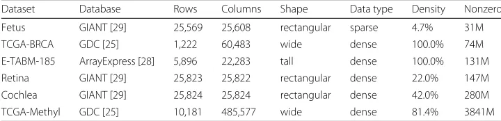
We considered the following six datasets (Table 1):

• TCGA-BRCA is an RNA-Seq gene expression dataset from the GDC databases [25].

The dataset contains expression measurements [26] of genes and gene variants from almost 1,300 human samples.

• E-TABM-185 is a microarray gene expression dataset [27] available at ArrayExpress

database with accession number E-TABM-185 [28]. It contains gene expression measurements from almost 6,000 human samples representing different cell and tissue types.

• Fetus denotes the fetus-specific functional interaction network from the GIANT

Table 1Summary of datasets

Dataset Database Rows Columns Shape Data type Density Nonzero Fetus GIANT [29] 25,569 25,608 rectangular sparse 4.7% 31M TCGA-BRCA GDC [25] 1,222 60,483 wide dense 100.0% 74M E-TABM-185 ArrayExpress [28] 5,896 22,283 tall dense 100.0% 131M Retina GIANT [29] 25,823 25,822 rectangular dense 22.0% 147M Cochlea GIANT [29] 25,824 25,824 rectangular dense 42.0% 280M TCGA-Methyl GDC [25] 10,181 485,577 wide dense 81.4% 3841M We manually categorized each data matrix into three shapes: tall datasets have substantially more rows than columns, wide datasets vice versa, and rectangular datasets have a comparable number of rows and columns. Density denotes the fraction of nonzero matrix elements. The number of nonzero elements in each matrix is given in the last column

• Retina denotes the retina-specific functional interaction network from the GIANT

database [29]. This is a network on human genes where two genes are connected if they are specifically co-expressed in retinal tissue. The retina-specific gene interaction network [31] has 147 million interactions.

• Cochlea denotes the cochlea-specific functional interaction network from the GIANT database [29]. This is a network on human genes where two genes are connected if they are specifically co-expressed in cochlear tissue. The

cochlea-specific gene interaction network [32] has 280 million interactions and is the densest network dataset in the GIANT database.

• TCGA-Methyl is a DNA methylation dataset from the GDC database [25], which

contains 10,181 samples from Illumina Human Methylation 450 platform [33]. Each sample contains methylation beta values for over 485,577 CpG sites.

Experimental setup

We factorized each dataset on multi-processor and on multi-GPU architectures. To asses the runtime statistics for a single iteration of factorization, factorization was run for 100 iterations, and measurements were averaged across ten runs. To test relationship between scalability and factorization rank, we varied parameterk, such thatk∈ {10, 20,. . ., 100}. For a given dataset and a given value of factorization rank, factor matrices were initialized to the same values across different platforms.

We considered the following runtime metrics:

• Speedupwas expressed as the ratio between processing timetAfor single iteration on

observed architectureA, and processing timetCPU−1on a single-CPU:sA= _tCPU−tA ₁.

• Efficiencywas expressed as a fraction of linear speedup, a speedup that assumes that

pprocessing units would reduce the runtime by a factor ofp. For an systemApwithp

processing units, we compute efficiency relative to performance of a single-unit systemA1on the same architecture. The formula is:EAp=

TA₁

pT_Ap. Efficiency of

EAp =1indicates a linear speedup. Communication cost pushes efficiency below this optimal value.

Implementation

uses OpenMPI [35] with Mpi4py Python interface [36]. Matrix operations are accelerated with OpenBLAS [37] on multi-processor architectures and CuBLAS [38] on GPUs. On multi-processor architectures we use NumPy for dense matrices and SciPy for opera-tions on sparse matrices. On GPUs we use Scikit-cuda [39] for dense matrix operaopera-tions and CuSPARSE [40] with Python-cuda-cffi [41] for operations on sparse matrices. Our implementation is available online [42].

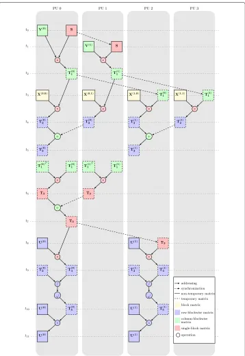
All experiments were run on a computational server with Intel Xeon E5-1650 proces-sor and on four NVIDIA Titan X (Maxwell) GPUs, each with 12 GB of memory. Givenp processing units, we split input data matrixXintopblocks, testing various block config-urations. Each block was passed to a processing unit that communicated the block with other units when data for next computational steps were required. Figure 3 shows an example of this computational and data transfer workflow for one update of matrixUon a 2×2-block configuration. Notice this workflow applies to both 4-GPU and 4-processor architecture.

Results

We here present results for non-orthogonal block-wise matrix tri-factorization. Results for orthogonal block-wise matrix tri-factorization are qualitatively the same and are provided in the Additional file 1.

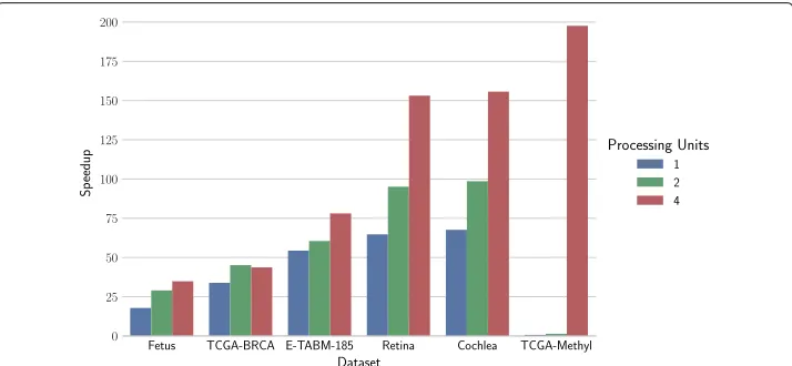
Figures 4 and 5 show speedups achieved on multi-processing and multi-GPU architec-tures, respectively, for each of six considered biomedical datasets. Runtime performance was tested on architectures with one, two or four processing units. Data matrices were partitioned according to block configurations in Table 2.

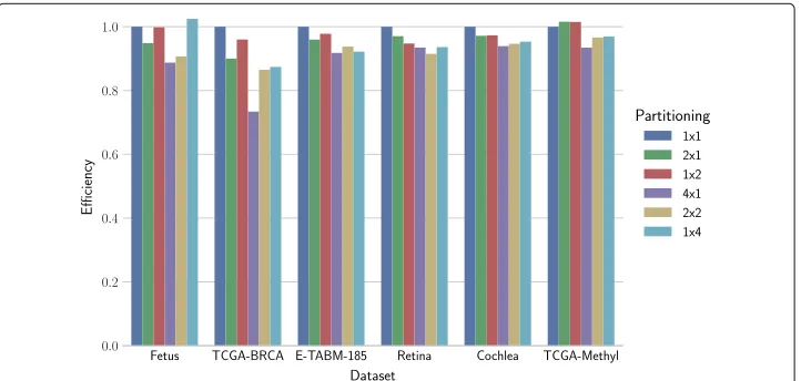
Efficiency of parallel implementation depends on dataset shape and on chosen block configuration. Measurements illustrating this dependency are shown in Fig. 6 for multi-processor architectures and in Fig. 7 for multi-GPU architectures.

One bottleneck of GPU-based architectures is communication overhead that occurs when copying data between GPU boards. This overhead was also observed in our experiments. For example, up to 50% of time needed to factorize TCGA-BRCA dataset in a 4-GPU environment was spent for communication. On larger datasets, however, this overhead was less pronounced. A detailed analysis is provided in Additional file 1: Figures S6 and S8. The communication overhead on multi-processor architectures is negligible as shown in the Additional file 1: Figures S5 and S7.

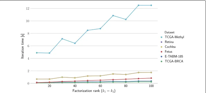
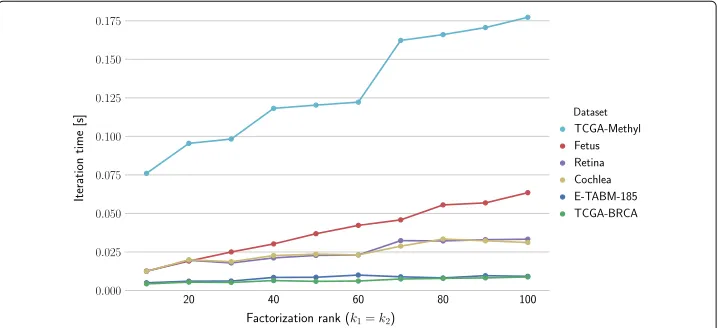
We also studied algorithm scalability with respect to factorization rank. Figure 9 shows runtime of one iteration as a function of factorization rank value on a four-GPU archi-tecture using a 2×2-block configuration. Figure 8 shows the results on a four-processor architecture.

Fig. 3Computational and data transfer workflow for block-wise update of factor matrixUon architecture with four processing units and data matrixXpartitioned into 2_×2 blocks. Each vertical band represents a processing unit (PU0 to PU3). Stages where all data are available for the next wave of asynchronous operations are horizontally aligned and are marked withti,i∈ {0, 1,. . ., 11}

Discussion Speedup

Fig. 4Computational speedups on multi-processing architectures. Speedup using 1, 2 and 4 processes compared to a configuration with one processor. Datasets are ordered from smallest to largest based on the number of non-zero values

elements, and we can observe a steady increase in speedup. Similar trends can also be observed on multi-processor architectures (Fig. 4), but the speedups are substantially lower than those on the GPUs.

For TCGA-Methyl dataset, the complete data matrix occupies about 19 GBytes of GPU’s memory (Additional file 1: Table S1). With a 12 GBytes of total memory on each GPU, and considering the overhead of libraries and temporary data matrices for inter-GPU communication, the data does not fit to the working memory in 1×1 and 1×2 block configurations. Running the factorization with 1×4 block configurations on 1-GPU or 2-GPU is feasible, but due to insufficient memory to store all necessary blocks in a single GPU requires a transfer of data between main memory and GPUs which severely impacts the runtime and prohibits any speedup. On this large dataset, a configuration with 4-GPUs has sufficient memory and provides for excellent speed-up (Fig. 5). This case also demonstrates that for large datasets the proposed approach

Table 2Block configurations used in experiments where we tested architectures with two or four processing units (PUs)

Dataset Data type 2 PUs 4 PUs

Fetus sparse 2×1 2×2

TCGA-BRCA dense 1×2 1×4

E-TABM-185 dense 2×1 4×1

Retina dense 2_×1 2_×2

Cochlea dense 2×1 2×2

TCGA-Methyl dense 1×2 (CPU only) 1×4

requires setups with the adequate number of GPUs that can keep all the data in working GPU memory.

Efficiency effects of block configuration

Block configuration plays a significant role in minimizing the impact of data transfers and balancing the load across devices (Figs. 6 and 7). Tall datasets (E-TABM-185) favor row-wise partitioning (e.g., 2×1 and 4×1). Wide datasets (TCGA-BRCA, TCGA-Methyl) favor column-wise partitioning (1×2 and 1×4). The two mentioned datasets, E-TABM-185 and TCGA-BRCA, are also those where the effect of the block configuration on efficiency was most pronounced. This observation highlights that suitable block configuration is data dependent, and also indicates that the selection of block configuration can be automated. The drop in efficiency under a particular choice of block configuration can be explained by increased communication overhead (Additional file 1: Figures S5 and S6). As we increase the number of devices that run in parallel, we need to perform additional data transfers that are not needed on setups with one matrix block. For example, in the case of tall dataset E-MTAB-185 and column-wise partitioning (1 × 4), over 40% of factorization runtime was spent for transferring data between GPUs. On the other hand, in the case of wide TCGA-BRCA dataset, the lowest efficiency was mea-sured when row-wise partitioning (4×1) was used, because communication cost was the highest.

Fig. 7Efficiency of multi-GPU architectures for different block configurations. Efficiency is represented by the fraction of linear speedup. The number of GPU devices is equal to the number of matrix blocks

Factorization rank

Next, we evaluate the performance of our approach when varying the value of the matrix factorization rank. Factorization rank is a vital parameter of all matrix factorization meth-ods because it determines the number of latent vectors. A larger factorization rank means the inferred latent model has a larger degree of freedom and can thus better approximate the input data matrix [43]. However, increasing factorization rank demands more com-putational resources and can result in poorer generalization performance [44]. Instead of determining the optimal factorization rank for a given dataset, our goal here is to investigate how the scalability of the proposed block-wise matrix factorization algorithm depends on the value of the factorization rank and on the sparsity of the input data matrix. Figure 8 shows the iteration time of NMTF as a function of factorization rank on a 4-processor architecture. We can observe that by increasing the factorization rank, the time of iteration increases linearly. For this analysis, both parametersk1 andk2, were

set with equal values and shown as a single factorization rank parameter. Partitioning

was done according to Table 2. When using a single process, the iteration time is proportionally slower according to the speedup shown in Fig. 4.

Figure 9 shows results that correspond to iteration time on 4-GPU architecture. We can see step-wise increases in iteration time, which is a result of the way the multiplication kernel utilizes the physical resources of the GPU [45]. The multiplication on the GPU is done on tiles of data which are processed by several threads in parallel. If the matrix shape is not aligned to the tile size, the border tiles will not make full use of the resources [46].

When comparing the factorization time of a sparse dataset (Fetus) and dense datasets (Retina, Cochlea) of similar size, the benefits of using sparse data structure are substantial. On a GPU, the factorization time on a sparse dataset (Fetus) is slower than on comparable dense datasets (Retina, Cochlea). This is because multiplication with sparse structures requires slower non-sequential memory access [47].

Interpretation of factorization results

Matrix factorization methods can be used to gain a better understanding of the data and their relationships as the methods identify cluster structures and detect potential new associations. The latent factors learned by NMTF reveal clusters in each of the two dimen-sions of the input data (matricesUandV) and encode cluster interactions (matrixS). The analysis of the latent factors can then lead to data interpretation, cluster discovery, and to prediction of new interactions.

We here demonstrate that tri-factorization can lead to the reconstruction of biologi-cally meaningful interactions. We have used a DNA methylation dataset (TCGA-Methyl, Table 1) consisting of 10,181 tissue samples from 33 cancer types. Tissue samples are pro-filed using methylation beta values for 485,577 CpG sites of the DNA. From these, we have considered only the sites that are related to 567 genes with known cancer interactions as listed in the Sanger cancer catalog [48]. Of those, 491 genes were included in our dataset and altogether involved 14,299 methylation sites. The resulting matrix had 10,181 rows and 14,299 columns. We factorized the matrix using factorization ranksk1=25,k2=30,

which yielded an optimal data compression with respect to the accuracy evaluated on a validation dataset (see Additional file 1: Figure S15).

Additional file 1: Table S2 lists five resulting cluster pairs that relate clusters of genes (from matrix V) and clusters of cancer types (from matrix U) with highest interaction scores in matrix S. First, we note that factorization revealed related cancer types, with, for example, colon, stomach and rectum adenocarcinoma (Additional file 1: Table S2, first row) forming its own group. Also, we found several com-mon Gene Ontology annotations for the clustered genes (Additional file 1: Table S3). Most importantly, we found evidence in published literature for a majority of inter-actions between genes and cancer types inferred through matrix tri-factorization.

For example, GATA2 was suggested as a prospective indicator for poor

prog-nosis in patients with colorectal cancer [49], and FAT4 functions as a tumor suppressor for stomach cancer [50]. Other supporting publications are listed in Additional file 1: Table S2.

Transcriptional silencing by DNA methylation plays an important role in the onset of cancer [51, 52]. It is thus encouraging that some of the critical interactions between methylated genes and diseases can be inferred, as demonstrated by this analysis, by non-negative matrix factorization of methylation cancer data alone.

Conclusion

Non-negative matrix tri-factorization is a successful modeling approach that can reveal hidden patterns in biomedical datasets. Current serial factorization approaches take sub-stantial runtime, particularly for larger datasets. We proposed a block-wise approach to speed up matrix tri-factorization through parallel execution. Experiments show the approach easily scales to very large datasets, and can achieve speedups of up to two orders of magnitude on current GPU-based architectures. We anticipate the proposed approach will be important for data integration, where matrix tri-factorization on large collections of data matrices [53] has already been proven superior and where execution times run into days.

Additional file

Additional file 1:Document with mathematical proofs, results for impact of communication, impact of balancing sparse datasets and results for orthogonal NMTF. (PDF 317 kb)

Abbreviations

CPU: Central processing unit; GPU: Graphics processing unit; MPI: Message passing interface; NMTF: Non-negative matrix tri-factorization; PU: Processing unit; RNA: Ribonucleic acid

Acknowledgements

This work was supported by Slovenian Research Agency grant P2-0209 and by a grant Health-F5-2010-242038 from European Union FP7 programme.

Availability of data and materials

A Python library implementing the proposed block-wise matrix tri-factorization is available at the GitHub repository https://github.com/acopar/crow.

Authors’ contributions

AC and MŽ developed the method; AC implemented the method and performed the experiments; and AC, MŽ and BZ wrote the manuscript. BZ coordinated the project. All authors read and approved the final manuscript.

Ethics approval and consent to participate

Competing interests

The authors declare that they have no competing interests.

Publisher’s Note

Springer Nature remains neutral with regard to jurisdictional claims in published maps and institutional affiliations.

Author details

1_{Faculty of Computer and Information Science, University of Ljubljana, Ljubljana, Slovenia.}2_{Department of Computer}

Science, Stanford University, Stanford, CA 94305, USA.3_{Baylor College of Medicine, Houston, TX 77030, USA.}

Received: 23 May 2017 Accepted: 4 December 2017

References

1. Lee DD, Seung HS. Algorithms for non-negative matrix factorization. In: Advances in Neural Information Processing Systems. Cambridge: MIT Press. 2001. p. 556–62.

2. Devarajan K. Nonnegative matrix factorization: an analytical and interpretive tool in computational biology. PLoS Comput Biol. 2008;4(7):1000029.

3. Lee CM, Mudaliar MA, Haggart D, Wolf CR, Miele G, Vass JK, Higham DJ, Crowther D. Simultaneous non-negative matrix factorization for multiple large scale gene expression datasets in toxicology. PloS ONE. 2012;7(12):48238. 4. Wang JJ-Y, Wang X, Gao X. Non-negative matrix factorization by maximizing correntropy for cancer clustering. BMC

Bioinformatics. 2013;14(1):107.

5. Northcott PA, Korshunov A, Witt H, Hielscher T, Eberhart CG, Mack S, Bouffet E, Clifford SC, Hawkins CE, French P, et al. Medulloblastoma comprises four distinct molecular variants. J Clin Oncol. 2010;29(11):1408–14.

6. Gönen M. Predicting drug–target interactions from chemical and genomic kernels using bayesian matrix factorization. Bioinformatics. 2012;28(18):2304–310.

7. Hwang T, Atluri G, Xie M, Dey S, Hong C, Kumar V, Kuang R. Co-clustering phenome–genome for phenotype classification and disease gene discovery. Nucleic Acids Res. 2012;40(19):146–6.

8. Sajda P, Du S, Brown TR, Stoyanova R, Shungu DC, Mao X, Parra LC. Nonnegative matrix factorization for rapid recovery of constituent spectra in magnetic resonance chemical shift imaging of the brain. IEEE Trans Med Imaging. 2004;23(12):1453–65.

9. Tikole S, Jaravine V, Rogov V, Dötsch V, Güntert P. Peak picking NMR spectral data using non-negative matrix factorization. BMC Bioinformatics. 2014;15(1):46.

10. Anderson A, Douglas PK, Kerr WT, Haynes VS, Yuille AL, Xie J, Wu YN, Brown JA, Cohen MS. Non-negative matrix factorization of multimodal MRI, fMRI and phenotypic data reveals differential changes in default mode

subnetworks in ADHD. NeuroImage. 2014;102:207–19.

11. Ding C, Li T, Peng W, Park H. Orthogonal nonnegative matrix t-factorizations for clustering. In: Proceedings of the 12th ACM SIGKDD International Conference on Knowledge Discovery and Data Mining. New York: ACM. 2006. p. 126–35.

12. Benson AR, Lee JD, Rajwa B, Gleich DF. Scalable methods for nonnegative matrix factorizations of near-separable tall-and-skinny matrices. In: Advances in Neural Information Processing Systems. Red Hook: Curran Associates, Inc. 2014. p. 945–53.

13. Kysenko V, Rupp K, Marchenko O, Selberherr S, Anisimov A. GPU-accelerated non-negative matrix factorization for text mining. In: International Conference on Application of Natural Language to Information Systems. Berlin: Springer. 2012. p. 158–63.

14. Platoš J, Gajdoš P, Krömer P, Snášel V. Non-negative matrix factorization on GPU. In: International Conference on Networked Digital Technologies. Berlin: Springer. 2010. p. 21–30.

15. Mejía-Roa E, Tabas-Madrid D, Setoain J, García C, Tirado F, Pascual-Montano A. NMF-mGPU: non-negative matrix factorization on multi-GPU systems. BMC Bioinformatics. 2015;16(1):43.

16. Sun Z, Li T, Rishe N. Large-scale matrix factorization using mapreduce. In: 2010 IEEE International Conference on Data Mining Workshops (ICDMW). Los Alamitos: IEEE Computer Society. 2010. p. 1242–8.

17. Dean J, Ghemawat S. Mapreduce: simplified data processing on large clusters. Commun ACM. 2008;51(1):107–13. 18. Yin J, Gao L, Zhang ZM. Scalable nonnegative matrix factorization with block-wise updates. In: Joint European

Conference on Machine Learning and Knowledge Discovery in Databases. Berlin: Springer. 2014. p. 337–52. 19. Long B, Zhang ZM, Yu PS. Co-clustering by block value decomposition. In: Proceedings of the Eleventh ACM

SIGKDD International Conference on Knowledge Discovery in Data Mining. New York: ACM. 2005. p. 635–40. 20. Ma C, Kamp Y, Willems LF. A frobenius norm approach to glottal closure detection from the speech signal. IEEE

Trans Speech Audio Process. 1994;2(2):258–65.

21. Guo S, Wu X, Li Y. On the lower bound of reconstruction error for spectral filtering based privacy preserving data mining. In: European Conference on Principles of Data Mining and Knowledge Discovery. Berlin: Springer. 2006. p. 520–7.

22. Zhang Y, Yeung DY. Overlapping community detection via bounded nonnegative matrix tri-factorization. In: Proceedings of the 18th ACM SIGKDD International Conference on Knowledge Discovery and Data Mining. New York: ACM. 2012. p. 606–14.

23. Chen G, Wang F, Zhang C. Collaborative filtering using orthogonal nonnegative matrix tri-factorization. Inf Process Manag. 2009;45(3):368–79.

24. Soni A, Jain S, Haupt J, Gonella S. Noisy matrix completion under sparse factor models. IEEE Trans Inf Theory. 2016;62(6):3636–61.

26. Lingle W, Erickson B, Zuley M, Jarosz R, Bonaccio E, Filippini J, Gruszauskas N. Radiology data from the cancer genome atlas breast invasive carcinoma [TCGA-BRCA] collection. The Cancer Imaging Archive. 2016. http://doi.org/ 10.7937/K9/TCIA.2016.AB2NAZRP. https://wiki.cancerimagingarchive.net/display/Public/TCGABRCA#

a1133e32f8c541859b2e9a19ec11c3cb. Accessed 12 Oct 2016.

27. Lukk M, Kapushesky M, Nikkilä J, Parkinson H, Goncalves A, Huber W, Ukkonen E, Brazma A. A global map of human gene expression. Nat Biotechnol. 2010;28(4):322–4.

28. Kolesnikov N, Hastings E, Keays M, Melnichuk O, Tang YA, Williams E, Dylag M, Kurbatova N, Brandizi M, Burdett T, et al. Arrayexpress update-simplifying data submissions. Nucleic Acids Res. 2014;43(D1):D1113–D1116. 29. Greene CS, Krishnan A, Wong AK, Ricciotti E, Zelaya RA, Himmelstein DS, Zhang R, Hartmann BM, Zaslavsky E, Sealfon SC, et al. Understanding multicellular function and disease with human tissue-specific networks. Nat Genet. 2015;47(6):569–76.

30. Fetus-specific functional interaction network. http://giant.princeton.edu/static/networks/fetus.gz. Accessed 10 Oct 2016.

31. Retina-specific functional interaction network. http://giant.princeton.edu/static/networks/retina.gz. Accessed 10 Oct 2016.

32. Cochlea-specific functional interaction network. http://giant.princeton.edu/static/networks/cochlea.gz. Accessed 10 Oct 2016.

33. GDC data portal. https://portal.gdc.cancer.gov/. Accessed 25 Sept 2017.

34. Klöckner A, Pinto N, Lee Y, Catanzaro B, Ivanov P, Fasih A. PyCUDA and PyOpenCL: a scripting-based approach to GPU run-time code generation. Parallel Comput. 2012;38(3):157–74.

35. Gabriel E, Fagg GE, Bosilca G, Angskun T, Dongarra JJ, Squyres JM, Sahay V, Kambadur P, Barrett B, Lumsdaine A, Castain RH, Daniel DJ, Graham RL, Woodall TS. Open MPI: Goals, concept, and design of a next generation MPI implementation. In: Proceedings, 11th European PVM/MPI Users’ Group Meeting. Berlin: Springer. 2004. p. 97–104. 36. Dalcin LD, Paz RR, Kler PA, Cosimo A. Parallel distributed computing using python. Adv Water Resources.

2011;34(9):1124–39.

37. Xianyi Z, Qian W, Yunquan Z. Model-driven level 3 BLAS performance optimization on loongson 3A processor. In: 18th IEEE International Conference on Parallel and Distributed Systems (ICPADS). Los Alamitos: IEEE Computer Society. 2012. p. 684–91.

38. CUDA Basic Linear Algebra Subroutines (cuBLAS). 2014. Available:https://developer.nvidia.com/cuBLAS. Accessed 13 June 2017.

39. Givon LE, Unterthiner T, Erichson NB, Chiang DW, Larson E, Pfister L, Dieleman S, Lee GR, van der Walt S, Moldovan TM, Bastien F, Shi X, Schlüter J, Thomas B, Capdevila C, Rubinsteyn A, Forbes MM, Frelinger J, Klein T, Merry B, Pastewka L, Taylor S, Wang F, Zhou Y. scikit-cuda 0.5.1: a Python interface to GPU-powered libraries. 2015. doi:10.5281/zenodo.40565. Accessed 27 Sept 2017.

40. NVIDIA CUDA Sparse Matrix library (cuSPARSE). 2010. Available: https://developer.nvidia.com/cusparse. Accessed 13 June 2017.

41. Lee GR. python-cuda-cffi repository. https://github.com/grlee77/python-cuda-cffi. Accessed 27 Sept 2017. 42. Copar A, Zitnik M, Zupan B. CROW: Fast Non-Negative Matrix Tri-Factorization. https://github.com/acopar/crow.

Accessed 27 Sept 2017.

43. Tan VY, Févotte C. Automatic relevance determination in nonnegative matrix factorization with theβ-divergence. IEEE Trans Pattern Anal Mach Intell. 2013;35(7):1592–605.

44. Kanagal B, Sindhwani V. Rank selection in low-rank matrix approximations: A study of cross-validation for NMFs. In: Proceedings of NIPS 2010: 6-11 December. Red Hook: Curran Associates, Inc. 2010.

45. Kurzak J, Tomov S, Dongarra J. Autotuning GEMM kernels for the fermi GPU. IEEE Trans Parallel Distributed Syst. 2012;23(11):2045–57.

46. Sørensen HHB. High-performance matrix-vector multiplication on the GPU. In: European Conference on Parallel Processing. Berlin: Springer. 2011. p. 377–86.

47. Monakov A, Lokhmotov A, Avetisyan A. Automatically tuning sparse matrix-vector multiplication for GPU architectures. In: International Conference on High-Performance Embedded Architectures and Compilers. Berlin: Springer. 2010. p. 111–25.

48. Futreal PA, Coin L, Marshall M, Down T, Hubbard T, Wooster R, Rahman N, Stratton MR. A census of human cancer genes. Nat Rev Cancer. 2004;4(3):177.

49. Xu K, Wang J, Gao J, Di J, Jiang B, Chen L, Wang Z, Wang A, Wu F, Wu W, et al. GATA binding protein 2 overexpression is associated with poor prognosis in KRAS mutant colorectal cancer. Oncol Rep. 2016;36(3):1672–8. 50. Cai J, Feng D, Hu L, Chen H, Yang G, Cai Q, Gao C, Wei D. FAT4 functions as a tumour suppressor in gastric cancer

by modulating wnt/β-catenin signalling. Br J Cancer. 2015;113(12):1720.

51. Luczak MW, Jagodzinski PP. The role of DNA methylation in cancer development. Folia Histochem Cytobiol. 2006;44(3):143–54.