Full Reference Objective Quality Assessment for Reconstructed Background Images

(1)

Full Reference Objective Quality Assessment

for Reconstructed Background Images

Aditee Shrotre1,∗,†,‡and Lina J. Karam1,†,‡

1 _{School of Electrical, Computer and Energy Engineering, Arizona State University, Tempe, AZ, 85287;} [email protected], [email protected]

* Correspondence: [email protected]; Tel.: +1-480-544-7216

† Current address: School of Electrical, Computer and Energy Engineering, Arizona State University, Tempe, AZ, 85287

‡ Aditee Shrotre and Lina Karam contributed to the design and development of the proposed method and to the writing of the manuscript. Aditee Shrotre contributed additionally to the software implementation and testing of the proposed method.

Abstract:With an increased interest in applications that require a clean background image, such as video surveillance, object tracking, street view imaging and location-based services on web-based maps, multiple algorithms have been developed to reconstruct a background image from cluttered scenes. Traditionally, statistical measures and existing image quality techniques have been applied for evaluating the quality of the reconstructed background images. Though these quality assessment methods have been widely used in the past, their performance in evaluating the perceived quality of the reconstructed background image has not been verified. In this work, we discuss the shortcomings in existing metrics and propose a full reference Reconstructed Background image Quality Index (RBQI) that combines color and structural information at multiple scales using a probability summation model to predict the perceived quality in the reconstructed background image given a reference image. To compare the performance of the proposed quality index with existing image quality assessment measures, we construct two different datasets consisting of reconstructed background images and corresponding subjective scores. The quality assessment measures are evaluated by correlating their objective scores with human subjective ratings. The correlation results show that the proposed RBQI outperforms all the existing approaches. Additionally, the constructed datasets and the corresponding subjective scores provide a benchmark to evaluate the performance of future metrics that are developed to evaluate the perceived quality of reconstructed background images.

Keywords: Background Reconstruction, Image Quality Assessment, Image Dataset, Subjective Evaluation, Perceptual Quality, Objective Quality Metric

1. Introduction

A clean background image has great significance in multiple applications. It can be used for video surveillance [1], activity recognition [2], object detection and tracking [3,4], street view imaging and location-based services on web-based maps [5,6], and texturing 3D models obtained from multiple photographs or videos [7]. But acquiring a clean photograph of a scene is seldom possible. There are always some unwanted objects occluding the background of interest. The technique of acquiring a clean background image by removing the occlusions using frames from a video or multiple views of a scene, is known as background reconstruction or background initialization. Many algorithms have been proposed for initializing the background images from videos, for example, [8–14]; and also from multiple images such as [15–17].

Background initialization or reconstruction is crippled by multiple challenges. The pseudo-stationary background (e.g., waving trees, waves in water, etc.) poses additional challenges in separating the moving foreground objects from the relatively stationary background pixels. The illumination conditions can vary across the images thus changing the global characteristics of each

(2)

the recovered image. Thus the background reconstruction algorithms can be characterized by two main tasks: 1. foreground detection, in which the foreground is separated from the background by classifying pixels as foreground or background; 2. background recovery, in which the holes formed due to foreground removal are filled.

The performance of a background extraction algorithm depends on two factors: 1. its ability to detect the foreground objects in the scene and completely eliminate them; and 2. the perceived quality of the reconstructed background image. Traditional statistical techniques such as Peak Signal to Noise Ratio (PSNR), Average Gray-level Error (AGE), total number of error pixels (EPs), percentage of EPs (pEP), number of Clustered Error Pixels (CEPs) and percentage of CEPs (pCEPs) [18] quantify the performance of the algorithm in its ability to remove foreground objects from a scene to a certain extent, but they do not give an indication of the perceived quality of the generated background image. On the other hand, the existing Image Quality Assessment (IQA) techniques such as Multi-scale Similarity metric (MS-SSIM) [19] and Color image Quality Measures (CQM) [20] used by the authors in [21] to compare different background reconstruction algorithms are not designed to identify any residual foreground objects in the scene. Lack of a quality metric that can reliably assess the performance of background reconstruction algorithms by quantifying both aspects of a reconstructed background image motivated the development of the proposed Reconstructed Background visual Quality Index (RBQI). The proposed RBQI is a full-reference objective metric that can be used by background reconstruction algorithm developers to assess and optimize the performance of their developed methods and also by users to select the best performing method. Research challenges such as the Scene Background Modeling Challenge (SBMC) 2016 [22] are also in need of a reliable objective scoring measure. RBQI uses the contrast, structure and color information to determine the presence of any residual foreground objects in the reconstructed background image as compared to the reference background image and to detect any unnaturalness introduced by the reconstruction algorithm that affects the perceived quality of the reconstructed background image.

This paper also presents two datasets that are constructed to assess the performance of the proposed as well as popular existing objective quality assessment methods in predicting the perceived visual quality of the reconstructed background images. The datasets consist of reconstructed background images generated using different background reconstruction algorithms in the literature along with the corresponding subjective ratings. Some of the existing datasets such as video surveillance datasets (Wallflower [23], I2R [24]), background subtraction datasets (UCSD [25], CMU [26]) and object tracking evaluation dataset (“Performance Evaluation of Tracking and Surveillance (PETS)") are not suited for this application as they do not provide reconstructed background images but just the foreground masks as ground-truth. The more recent dataset “Scene Background Modeling Net" (SBMNet) [27] is targeted at comparing the performance of the background initialization algorithms but it does not provide any subjective ratings for the reconstructed background images. Hence the SBMNet dataset [27] is not suited for benchmarking the performance of objective background visual quality assessment. The datasets proposed in this work are the first and currently the only datasets that can be used for benchmarking existing and future metrics developed to assess the quality of reconstructed background images.

(3)

for reconstructed background images. Finally, we conclude the paper in Section6and also provide directions for future research.

2. Existing Full Reference Background Quality Assessment Techniques and their Limitations

Existing background reconstruction quality metrics can be classified into two categories: statistical and image quality assessment (IQA) techniques, depending on the type of features used for measuring the similarity between the reconstructed background image and reference background image.

2.1. Statistical Techniques

Statistical techniques use intensity values at co-located pixels in the reference and reconstructed background images to measure the similarity. Popular statistical techniques [18] that have been traditionally used for judging the performance of background initialization algorithms are briefly explained here.

(i) Average Gray-level Error (AGE): AGE is calculated as the absolute difference between the gray levels of the co-located pixels in the reference and reconstructed background image.

(ii) Error Pixels (EP): EPgives the total number of error pixels. A pixel is classified as an error pixel if the absolute difference between the corresponding pixels in the reference and reconstructed background images is greater than an empirically selected thresholdτ.

(iii) Percentage Error Pixels (pEP): Percentage of the error pixels, calculated asEP/N, whereNis the total number of pixels in the image.

(iv) Clustered Error Pixels (CEP):CEPgives the total number of clustered error pixels. A clustered error pixel is defined as the error pixel whose 4 connected pixels are also classified as error pixels. (v) Percentage Clustered Error Pixels (pCEP): Percentage of the clustered error pixels, calculated as CEP/N, whereNis the total number of pixels in the image.

Though these techniques have been used to judge the quality of the reconstructed background images, their performance has not been previously evaluated. As we show in Section5and as noted by the authors in [28], the statistical techniques were found to not correlate well with the subjective quality scores.

2.2. Image Quality Assessment Techniques

The existing Full Reference Image Quality Assessment (FR-IQA) techniques use perceptually inspired features for measuring the similarity between two images. Though these techniques have been shown to work reasonably well while assessing images affected by distortions such as blur, compression artifacts and noise, these techniques have not been designed for assessing the quality of reconstructed background images. In [21] popular FR-IQA techniques including Peak Signal to Noise Ratio (PSNR), Multi-Scale Similarity (MS-SSIM) [19] and Color image Quality Measure (CQM) [20], were adopted for objectively comparing the performance of the different background reconstruction algorithms; however, no performance evaluation was carried out to support the choice of these techniques. Other popular IQA techniques include Structural Similarity Index (SSIM) [29], visual signal-to-noise ratio (VSNR) [30], visual information fidelity (VIF) [31], pixel-based VIF (VIFP) [31], universal quality index (UQI) [32], image fidelity criterion (IFC) [33], noise quality measure (NQM) [34], weighted signal-to-noise ratio (WSNR) [35], feature similarity index (FSIM) [36], FSIM with color (FSIMc) [36], spectral residual based similarity (SR-SIM) [37] and saliency-based SSIM (SalSSIM) [38]. The suitability of these techniques for evaluating the quality of reconstructed background images remains unexplored.

(4)

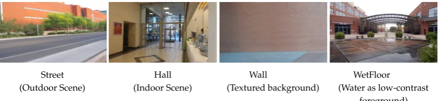
Street (Outdoor Scene)

Hall (Indoor Scene)

Wall

(Textured background)

WetFloor

(Water as low-contrast foreground)

(a)Scenes with static backgrounds from the ReBaQ dataset.

Building (Reflective)

Escalator (Large Motion)

llumination

(Illumination Variations)

Park (Small Motion)

(b)Scenes with pseudo-stationary backgrounds from the ReBaQ dataset.

Figure 1.Reference background images for different scenes in the Reconstructed Background Quality (ReBaQ) Dataset. Each reference background image corresponds to a captured scene background without foreground objects.

well with the subjective scores as discussed in Section5. This motivated our second contribution, the objective Reconstructed Background Quality Index (RBQI) that is shown to outperform all the existing techniques in assessing the perceived visual quality of reconstructed background images.

3. Subjective Quality Assessment of Reconstructed Background Images

3.1. Datasets

In this section we present two different datasets constructed as part of this work to serve as benchmarks for comparing existing and future techniques developed for assessing the quality of reconstructed background images. The images and subjective experiments for both datasets are described in the subsequent subsections.

Each dataset contains the original sequence of images or videos that are used as inputs to the different reconstruction algorithms, the background images reconstructed by the different algorithms and the corresponding subjective scores.

3.1.1. Reconstructed Background Quality (ReBaQ) Dataset

This dataset consists of eight different scenes. Each scene consists of a sequence of 8 images where every image is a different view of the scene captured by a stationary camera. Each image sequence is captured such that the background is visible at every pixel in at least one of the views. A reference background image that is free of any foreground objects is also captured for every scene. Figure1 shows the reference images corresponding to each of the eight different scenes in this dataset. The spatial resolution of the sequence corresponding to each of the scenes is 736x416.

(5)

quality of the recovered background. As a result, 18 background images are generated for each of the 8 scenes. These 144(18×8)reconstructed background images along with the corresponding reference images for the scene are then used for the subjective evaluation. Each of the scenes pose a different challenge for the background reconstruction algorithms. For example, “Street” and “Wall” are outdoor sequences with textured backgrounds while “Hall” is an indoor sequence with textured background. The “WetFloor” sequence challenges the underlying principal of many background reconstruction algorithms with water appearing as a low-contrast foreground object. The “Escalator” sequence has large motion in the background due to the moving escalator, while “Park” has smaller motion in the background due to waving trees. The “Illumination” sequence exhibits changing light sources, directions and intensities while the “Building” sequence has changing reflections in the background. Broadly, the dataset contains two categories based on the scene characteristics: (i) Static, the scenes for which all the pixels in the background are stationary; and (ii) Dynamic, the scenes for which there are non-stationary background pixels (e.g., moving escalator, waving trees, varying reflections). Four out of the eight scenes in the ReBaQ dataset are categorized as Static and the remaining four are categorized as Dynamic scenes. The reference background images corresponding to the static scenes are shown in Figure1(a). Although there are reflections on the floor in the “WetFloor” sequence, it does not exhibit variations at the time of recording and hence it is categorized as a static background scene. The reference background images corresponding to the dynamic background scenes are shown in Figure1(b).

3.1.2. SBMNet based Reconstructed Background Quality (S-ReBaQ) Dataset

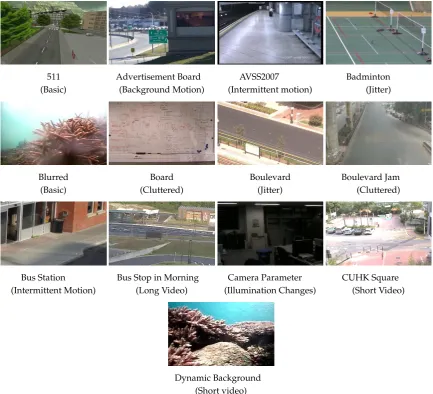
This dataset is created from the videos in the Scene Background Modeling Net (SBMNet) dataset [27] used for the Scene Background Modeling Challenge (SBMC) 2016 [22]. SMBNet consists of image sequences corresponding to a total of 79 scenes. These image sequences are representative of typical indoor and outdoor visual data captured in surveillance, smart environment, and video dataset scenarios. The spatial resolutions of the sequences corresponding to different scenes vary from 240x240 to 800x600. The length of the sequences also varies from 6 to 9,370 images. The authors of SBMNet categorize these scenes into eight different classes based on the challenges posed [27]: (a) Basic category represents a mixture of mild challenges typical of the shadows, Dynamic Background, Camera Jitter and Intermittent Object Motion categories; (b) Background motion category includes scenes with strong (parasitic) background motion; for example, in the “Advertisement Board” sequence the advertisement board in the scene periodically changes; (c) Intermittent Motion category includes sequences with scenarios known for causing “ghosting” artifacts in the detected motion; (d) Jitter category contains indoor and outdoor sequences captured by unstable cameras; (e) Clutter category includes sequences containing a large number of foreground moving objects occluding a large portion of the background; (f) Illumination Changes category contains indoor sequences containing strong and mild illumination changes; (g) Very Long category contains sequences each with more than 3,500 images; (h) Very Short category contains sequences with a limited number of images (less than 20). The authors of SBMNet [27] provide reference background images for only 13 scenes out of the 79 scenes. There is at least one scene corresponding to each category with reference background image available. We use only these 13 scenes for which the reference background images are provided. Figure2shows the reference background images corresponding to the scenes in this dataset with the categories from SBMNet [27] in brackets. Background images that were reconstructed by 14 algorithms submitted to SBMC [12,16,39–48] corresponding to the selected 13 scenes were used in this work for conducting subjective tests. As a result, a total of 182 (13×14) reconstructed background images along with their corresponding subjective scores form the S-ReBaQ dataset.

3.2. Subjective Evaluation

(6)

511 (Basic)

Advertisement Board (Background Motion)

AVSS2007 (Intermittent motion)

Badminton (Jitter)

Blurred (Basic)

Board (Cluttered)

Boulevard (Jitter)

Boulevard Jam (Cluttered)

Bus Station (Intermittent Motion)

Bus Stop in Morning (Long Video)

Camera Parameter (Illumination Changes)

CUHK Square (Short Video)

Dynamic Background (Short video)

Figure 2. Reference background images for different scenes in the SBMNet based Reconstructed Background Quality (S-ReBaQ) Dataset. Each reference background image corresponds to a captured scene background without foreground objects.

(7)

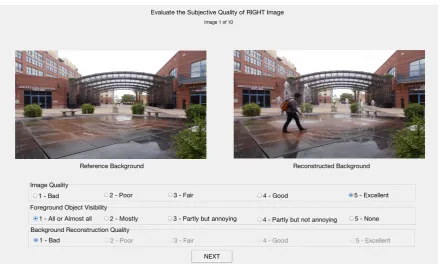
Figure 3.Subjective test Graphical User Interface (GUI).

referred to as raw scores in the rest of the paper, are used for calculating the Mean Opinion Score (MOS).

We adopted a double-stimulus technique in which the reference and the reconstructed background images were presented side-by-side [49] to each subject as shown in Figure3. Though the same testing strategy and set up was used for the ReBaQ and S-ReBaQ datasets described in Section3.1, the tests for each dataset were conducted in separate sessions.

As discussed in [28], the subjective experiments were carried out on a 23-inch Alienware monitor with a resolution of 1920x1080. Before the experiment, the monitor was reset to its factory settings. The setup was placed in a laboratory under normal office illumination conditions. Subjects were asked to sit at a viewing distance of 2.5 times the monitor height.

Seventeen subjects participated in the subjective test for the ReBaQ dataset, while sixteen subjects participated in the subjective test for the S-ReBaQ dataset. The subjects were tested for vision and color blindness using the Snellen chart [50] and Ishihara color vision test [51], respectively. A training session was conducted before the actual subjective testing, in which the subjects were shown few images covering different quality levels and distortions of the reconstructed background images and their responses were noted to confirm their understanding of the tests. The images used during training were not included in the subjective tests.

(8)

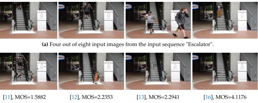
(a)Four out of eight input images from the input sequence "Escalator".

[11], MOS=1.5882 [12], MOS=2.2353 [13], MOS=2.2941 [16], MOS=4.1176

(b)Background images reconstructed by different algorithms and corresponding MOS scores.

Figure 4.Example input sequence and recovered background images with corresponding MOS scores from the ReBaQ dataset.

Figure4shows an input sequence for a scene in the ReBaQ dataset together with reconstructed background images using different algorithms and corresponding MOS scores.

4. Proposed Reconstructed Background Quality Index

In this section we propose a full-reference quality index that can automatically assess the perceived quality of the reconstructed background images. The proposed Reconstructed Background Quality Index (RBQI) uses a probability summation model to combine visual characteristics at multiple scales and quantify the deterioration in the perceived quality of the reconstructed background image due to the presence of any residual foreground objects or unnaturalness that may be introduced by the background reconstruction algorithm. The motivation for RBQI comes from the fact that the quality of a reconstructed background image depends on two factors namely: (i) the visibility of the foreground objects, and (ii) the visible artifacts introduced while reconstructing the background image.

A block diagram of the proposed quality index (RBQI) is shown in Figure5. AnL-level multi-scale decomposition of the reference and reconstructed background images is obtained through lowpass filtering using an averaging filter [19] and downsampling, wherel=0 corresponds to the finest scale andl = L−1 corresponds to the coarsest scale. For each levell = 0, ...,L−1, contrast, structure and color differences are computed locally at each pixel to produce a contrast-structure difference map and a color difference map. The difference maps are combined in local regions within each scale and later across scales using a ‘probability summation model’ to predict the perceived quality of the reconstructed background image. More details about the computation of the difference maps and the proposed RBQI based on a probability summation model are provided below.

4.1. Structure Difference Map (ds)

(9)

Reference background image

at scale l

Reconstructed background image

at scale l

Compute block distortion DR using eq.(18) and eq.(19)

Is l < L?

Compute RBQI as logarithm of _Dlpooled over all scales

using eq.(29) and eq.(31) Yes Yes

No Compute: ds,l using eq.(4) dc,l using eq.(5)

Compute level distortion Dl using eq.(22) and eq.(23)

Go to next scale

l++

Go to next scale

l++

Figure 5. Block diagram describing the computation of the proposed Reconstructed Background Quality Index (RBQI).

background images, calculated at each pixel, give us the ‘contrast-structure difference map’ referred to as ‘structure map’ for short in the rest of the paper.

First the structure similarity between the reference and the reconstructed background image, referred to as Structure Index (SI), is calculated using [29]:

SI(x,y) = 2σr(x,y)i(x,y)+C

σ_r2 (x,y)+σ

2 i(x,y)+C

(1)

whereris the reference background image,iis the reconstructed background image,σrandσiare the

standard deviations of the reference and reconstructed background image, respectively.σr(x,y),i(x,y)is

the cross-correlation between the reference and reconstructed background images at location(x,y).C is a small constant to avoid instability and is calculated asC= (K·Imax)2,Kis set to 0.03 andImaxis

the maximum possible value of the pixel intensity (255 in this case) [29]. A higherSIvalue indicates higher similarity between the pixels in the reference and reconstructed background images.

The background scenes often contain pseudo-stationary objects such as waving trees, escalator, local and global illumination changes. Even though these pseudo-stationary pixels belong to the background, because of the presence of motion, they are likely to be classified as foreground pixels. For this reason the pseudo-stationary backgrounds pose an additional challenge for the quality assessment algorithms. Just comparing co-located pixel neighborhoods in the two considered images is not sufficient in the presence of such dynamic backgrounds, our algorithm uses a search window of size nhood×nhoodcentered at the current pixel(x,y)in the reconstructed image, wherenhoodis an odd value. TheSI is calculated between the pixel at location(x,y)in the reference image and(nhood)2

(10)

(a)scalel=0 (b)scalel=1 (c)scalel=2

Figure 6.Structure Index (SI) map withnhood=17 for the background image shown in Figure4(b) and reconstructed using the method in [12]. The darker regions indicate larger structure differences between the reference and the reconstructed background image.

SI₍_x_,_y₎(m,n) = 2σr(x,y)i(m,n) +C

σ_r2 (x,y)+σ

2 i(m,n)+C

(2)

where

m=x−(nhood−1)/2 :x+ (nhood−1)/2 n=y−(nhood−1)/2 :y+ (nhood−1)/2

The maximum value of theSImatrix is taken to be the finalSIvalue for the pixel at location(x,y)as given below:

SI(x,y) =max

(m,n)(SI(x,y)(m,n)) (3) TheSImap takes on values between [-1,1].

In the proposed method, theSImap is computed atLdifferent scales denoted asSIl(x,y),l =

0, ...,L−1. The SImaps generated at three different scales for the background image shown in Figure4(b)and reconstructed using the method of [12] are shown in Figure6. The darker regions in these images indicate larger structure differences between the reference and the reconstructed background images while the lighter regions indicate higher similarities.

The structure difference map is calculated using theSImap at each scalelas follows:

ds,l(x,y) =1

−SIl(x,y)

2 (4)

ds,ltakes on values between [0,1] where the value of 0 corresponds to no difference while 1 corresponds

to largest difference.

4.2. Color Distance (dc)

Theds,lmap is vulnerable to failures while detecting differences in areas of background images

(11)

color information at every scale while calculating the RBQI. The color difference between the filtered reference and reconstructed background images at each scalel is then calculated as the Euclidian distance between the values of co-located pixels as follows:

dc,l(x,y) =

q

(Lr(x,y)−Li(x,y))2+ (ar(x,y)−ai(x,y))2+ (br(x,y)−bi(x,y))2 (5)

4.3. Computation of the Reconstructed Background Quality Index (RBQI) based on Probability Summation As indicated previously, the reference and reconstructed background images are decomposed each into a multi-scale pyramid withLlevels. Structure difference mapsds,land color difference maps

dc,lare computed at every levell=0, ...,L−1 as described in Equations (4) and (5), respectively. These

difference maps are pooled together within the scale and later across all scales using a probability summation model [52] to give the final RBQI.

The probability summation model as described in [52] considers an ensemble of independent difference detectors at every pixel location in the image. These detectors predict the probability of perceiving the difference between the reference and the reconstructed background images at the corresponding pixel location based on its neighborhood characteristics in the reference image. Using this model, the probability of the structure difference detector signaling the presence of a structure difference at pixel location(x,y)at levellcan be modeled as an exponential of the form:

PD,s,l(x,y) =1−exp −

ds,l(x,y) αs,l(x,y)

βs! (6)

where βs is a parameter chosen to increase the correspondence of RBQI with the experimentally

determined MOS scores on a training dataset andαs,l(x,y)is a parameter whose value depends upon

the texture characteristics of the neighborhood centered at(x,y)in the reference image. The value ofαs,l(x,y)is chosen to take into account that differences in structure are less perceptible in textured

areas as compared to non-textured areas and that the perception of these differences depends on the scalel.

In order to determine the value ofαs,l, every pixel in the reference background image at scalel

is classified as textured or non-textured using the technique in [53]. This method first calculates the local variance at each pixel using a 3x3 window centered around it. Based on the computed variances a pixel is classified as edge, texture or uniform. By considering the number of edge, texture and uniform pixels in the 8x8 neighborhood of the pixel, it is further classified into one of the six types: uniform, uniform/texture, texture, edge/texture, medium edge and strong edge. For our application we label the pixels classified as ‘texture’ and ‘edge/texture’ as ’textured’ pixels and we label the rest as ‘non-textured’ pixels.

Letftex,l(x,y) =1 be the flag indicating that a pixel is textured. Thus values ofαs,l(x,y)can be

expressed as:

αs,l(x,y) =

(

1.0, if ftex,l(x,y) =0

a, wherea1.0, if ftex,l(x,y) =1

(7)

In our implementation we chose the value ofa=1000.0.

Similarly, the probability of the color difference detector signaling the presence of a color difference at pixel location(x,y)at levellcan be modeled as:

PD,c,l(x,y) =1−exp −

dc,l(x,y) αc,l(x,y)

βc! (8)

whereβcis found in a similar way toβs andαc,l(x,y)corresponds to the Adaptive Just Noticeable

(12)

(x,y)in the Lab color space,JNCDLabis set to 2.3 [55],E(Ll)is the mean background luminance of the

pixel at(x,y)and∆Lis the maximum luminance gradient across pixel(x,y). In Equation (9),sCis the

scaling factor used for adjusting the dimension of ellipsoid along the chroma axis as is given by [54]:

sC(al(x,y),bl(x,y)) =1+0.045·(a2l(x,y) +b2l(x,y))1/2 (10)

sLis the scaling factor that simulates the local luminance texture masking and is given by:

sL(E(Ll),∆Ll) =ρ(E(Ll))∆Ll+1.0 (11)

whereρ(E(Ll))is the weighting factor as described in [54]. Thus,αc,l varies at every pixel location

based on the distance between the chroma values and texture masking properties of its neighborhood. A pixel(x,y)at thel-th level is said to have no distortion if and only if neither the structure difference detector nor the color difference detector at location(x,y)signal the presence of a difference. Thus, the probability of detecting no difference between the reference and reconstructed background images at pixel(x,y)and levellcan be written as:

PND,l(x,y) = (1−PD,s,l(x,y))·(1−PD,c,l(x,y)) (12)

Substituting Equation (6) and Equation (8) forPD,s,landPD,c,l, respectively, in Equation (12), we get:

PND,l(x,y) =exp(−Ds,l(x,y))·exp(−Dc,l(x,y)) (13)

where

Ds,l(x,y) =

βs

(14)

and

Dc,l(x,y) =

dc,l(x,y) α_c_,_l(x,y)

βc

(15)

A less localized probability of difference detection can be computed by adopting the “probability summation” hypothesis [52] which pools the localized detection probabilities over a regionR. The probability summation hypothesis is based on the following two assumptions: 1)Assumption 1: A structure difference is detected in the region of interestRif and only if at least one detector inRsignals the presence of a difference, i.e., if and only if at least one of the differencesds,l(x,y)is above threshold αsand, therefore, considered to be visible. Similarly, a color difference is detected in regionRif and

only if at least one of the differencesdc,l(x,y)is aboveαc.

2)Assumption 2:The probabilities of detection are independent; i.e., the probability that a particular detector will signal the presence of a difference is independent of the probability that any other detector will. This simplified approximation model is commonly used in the psychophysics literature [52,56] and was found to work well in practice in terms of correlation with human judgement in quantifying perceived visual distortions [57,58].

Then the probability of no difference detection over the regionRis given by: PND,l(R) =

∏

(x,y)∈R

(13)

Substituting Equation (12) in the above equation gives:

PND,l(R) =exp −Ds,l(R)βs

·exp −Dc,l(R)βc

(17)

where

Ds,l(R) =

∑

(x,y)∈R

βs!_β1_s

(18)

Dc,l(R) =

∑

(x,y)∈R

dc,l(x,y) α_c_,_l(x,y)

βc!_β1_c

(19)

In the human visual system, the highest visual acuity is limited to the size of the foveal region, which covers approximately 2◦ of visual angle. In our work, we consider the image regionsRas foveal regions approximated by 8×8 non-overlapping image blocks.

The probability of no distortion detection over thel-th level is obtained by pooling the no detection probabilities over all the regionsRin levelland is given by:

PND(l) =

∏

R∈l

PND,l(R) (20)

or

PND(l) =exp −Ds(l)βs·exp −Dc(l)βc (21)

where

Ds(l) =

∑

R∈l

Ds,l(R)βs

_β1_s

(22)

Dc(l) =

∑

R∈l

Dc,l(R)βc

_β1_c

(23)

Similarly, we adopt a “probability summation” hypothesis to pool the detection probability across scales. The Human Visual Systems (HVS) dependent parametersα_s_,_l andα_c_,_l that are included in

Equations (14) and (15), respectively, account for the varying sensitivity of the HVS at varying scales. The final probability of detecting no distortion in a reconstructed background imageiis obtained when no distortion is detected at any scale and is computed by pooling the no detection probabilitiesPND(l)

over all scalesl,l=0, ...,L−1, as follows:

PND(i) = L−1

∏

l=0

PND(l) (24)

or

PND(i) =exp −Dsβs·exp −Dcβc (25)

where

Ds =

L−1

∑

l=0

Ds(l)βs

_β1_s

(26)

Dc=

L−1

∑

l=0

Dc(l)βc

_β1_c

(27)

whereDs(l)andDc(l)are given by Equations (22) and (23), respectively. From Equations (26) and (27),

(14)

where

D=

L−1

∑

l=0R

∑

∈l(x,

∑

y)∈R

Ds,l(x,y) +Dc,l(x,y)

(29)

In Equation (29),Ds,l(x,y)andDc,l(x,y)are given by Equations (14) and (15), respectively. Thus the

probability of detecting a difference between the reference image and a reconstructed background imageiis given as:

PD(i) =1−PND(i) =1−exp(−D) (30)

As it can be seen from Equation (30), a lower value ofDresults in a lower probability of difference detectionPD(i)while a higher value results in a higher probability of difference detection. Therefore,

Dcan be used to assess the perceived quality in the reconstructed background image, with a lower value ofDcorresponding to a higher perceived quality.

The final Reconstructed Background Quality Index (RBQI) for a reconstructed background image is calculated using the logarithm ofDas follows:

RBQI=log₁₀(1+D) (31)

AsDincreases the value of RBQI increases implying more perceived distortion and thus lower quality of the reconstructed background image. The logarithmic mapping models the saturation effect, i.e., beyond a certain point the maximum annoyance level is reached and more distortion does not affect the quality.

5. Results

In this section we analyze the performance of RBQI in terms of its ability to predict the subjective ratings for the perceived quality of reconstructed background images. We evaluate the performance of the proposed quality index in terms of its prediction accuracy and prediction monotonicity and provide comparisons with the existing statistical and IQA techniques. In our implementation, we setnhood=17,L=3,βs =βc=3.5. We also evaluate the performance of RBQI for different scales

(15)

Table 1.Comparison of RBQI vs. Statistical measures and IQA techniques on the ReBaQ dataset.

(a)Comparison on the ReBaQ-Static dataset.

ReBaQ-Static

PCC SROCC RMSE OR PPCC PSROCC

Statistical Measur

es AGE 0.7776 0.6348 0.6050 9.72% 0.000000 0.000000 EPs 0.3976 0.5093 0.8829 13.89% 0.000000 0.000000 pEPs 0.8058 0.6170 0.5698 6.94% 0.000000 0.000000 CEPs 0.5719 0.6939 0.7893 11.11% 0.000000 0.000000 pCEPs 0.6281 0.7843 0.9622 13.89% 0.000000 0.000000

Image

Quality

Assessment

Metrics

PSNR 0.8324 0.7040 0.5331 8.33% 0.000000 0.000000 SSIM[29] 0.5914 0.5168 0.7759 11.11% 0.000000 0.000177 MS-SSIM[19] 0.7230 0.7085 0.6648 8.33% 0.000000 0.000000 VSNR[30] 0.5216 0.3986 0.8209 9.72% 0.000003 0.000531 VIF[31] 0.3625 0.0843 0.8968 15.28% 0.001754 0.484429 VIFP[31] 0.5122 0.3684 0.8265 11.11% 0.000004 0.001470 UQI[32] 0.6197 0.7581 0.9622 13.89% 0.000000 0.000000 IFC[33] 0.5003 0.3771 0.8331 11.11% 0.000008 0.001105 NQM[34] 0.8251 0.8602 0.5437 6.94% 0.000000 0.000000 WSNR[35] 0.8013 0.7389 0.5756 5.56% 0.000000 0.000000 FSIM[36] 0.7209 0.6970 0.6668 9.72% 0.000000 0.000000 FSIMc[36] 0.7274 0.7033 0.6603 9.72% 0.000000 0.000000 SRSIM[37] 0.7906 0.7862 0.5892 8.33% 0.000000 0.000000 SalSSIM[38] 0.5983 0.5217 0.7710 9.72% 0.000000 0.000003 CQM[20] 0.6401 0.5755 0.7393 8.33% 0.000000 0.000000 RBQI(Proposed) 0.9006 0.8592 0.4183 4.17% 0.000000 0.000000

(b)Comparison on the ReBaQ-Dynamic dataset.

ReBaQ-Dynamic

Statistical Measur

es AGE 0.4999 0.2303 0.7644 9.72% 0.005000 0.051600 EPs 0.1208 0.2771 0.8761 13.89% 0.007600 0.018500 pEPs 0.4734 0.2771 0.8825 9.72% 0.007600 0.018500 CEPs 0.5951 0.7549 0.7092 11.11% 0.000000 0.000000 pCEPs 0.6418 0.7940 0.8826 15.28% 0.000000 0.000000

Image

Quality

Assessment

Metrics

(16)

Statistical Measur

Image

Quality

Assessment

Metrics

PSNR 0.7099 0.6834 0.7686 6.59% 0.000000 0.000000 SSIM[29] 0.5975 0.5827 0.8751 12.09% 0.000000 0.000000 MS-SSIM[19] 0.8048 0.8030 0.6478 29.12% 0.000000 0.000000 VSNR[30] 0.0850 0.1717 1.0874 13.19% 0.253675 0.486686 VIF[31] 0.1027 0.2064 1.0914 27.47% 0.167842 0.005305 VIFP[31] 0.6081 0.6240 0.8664 26.92% 0.000000 0.000000 UQI[32] 0.6316 0.5932 0.8461 14.84% 0.000000 0.000000 IFC[33] 0.6235 0.6020 0.8533 16.48% 0.000000 0.000000 NQM[34] 0.7950 0.7816 0.6621 14.84% 0.000000 0.000000 WSNR[35] 0.7176 0.6888 0.7601 7.14% 0.000000 0.000000 FSIM[36] 0.7243 0.7157 0.7525 10.44% 0.000000 0.000000 FSIMc[36] 0.7278 0.7172 0.7484 12.09% 0.000000 0.000000 SRSIM[37] 0.7853 0.7538 0.6757 12.09% 0.000000 0.000000 SalSSIM[38] 0.7356 0.7300 0.7393 7.14% 0.000000 0.000000 CQM[20] 0.2634 0.3645 1.0531 8.24% 0.000327 0.000276 RBQI(Proposed) 0.8613 0.8222 0.5545 3.30% 0.000000 0.000000

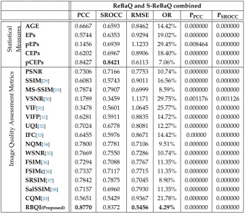
Table 3.Comparison of RBQI vs. Statistical measures and IQA techniques on a combined ReBaQ and S-ReBaQ dataset.

ReBaQ and S-ReBaQ combined

Statistical Measur

Image

Quality

Assessment

Metrics

(17)

We use the two datasets ReBaQ and S-ReBaQ described in Section3.1to quantify and compare the performance of RBQI. For performance evaluation, we employ three most commonly used metrics: (i) Spearman rank-order correlation coefficient (SROCC); (ii) Pearson correlation coefficient (PCC); and (iii) root mean squared error (RMSE). A 4-parameter regression function [59] is applied to the IQA metrics to provide a non-linear mapping between the objective scores and the subjective mean opinion scores (MOS):

MOSpi =

γ1−γ2

1+e−

Mi−γ₃

|γ₄|

+γ2 (32)

whereMidenotes the predicted quality for theith image andMOSpi denotes the quality score after

fitting, andγn,n=1, 2, ..., 4, are the regression model parameters. MOSpi along with MOS scores are

used to calculate the PCC values given in the Tables1,2and3.

5.1. Performance Comparison

Tables1and2show the obtained performance evaluation results of the proposed RBQI technique on the ReBaQ and S-ReBaQ datasets, respectively, as compared to the existing statistical and FR-IQA algorithms. The results show that the proposed quality index yields higher correlation with the subjective scores as compared to any other existing technique. The statistical techniques are shown to not correlate well with the subjective scores on either of the datasets. Among the FR-IQA algorithms, the performance of the NQM [34] comes close to the proposed technique for scenes with static background images, i.e., for the ReBaQstaticdataset, as it considers the effects of contrast sensitivity,

luminance variations, contrast interaction between spatial frequencies and contrast masking effect while weighting the SNR between the ground truth and reconstructed image. The more popular MS-SSIM [19] technique is shown to not correlate well with the subjective scores for the ReBaQ dataset. This is because the MS-SSIM calculates the final quality index of the image by just averaging over the entire image. In the problem of background reconstruction the error might occupy a relatively small area as compared to the image size, thereby under-penalizing the residual foreground. None of the FR-IQA or statistical techniques were found to correlate with the scores in the ReBaQdynamicdataset.

This is because the assumption of pixel-to-pixel correspondence is no longer valid in the presence of pseudo-stationary background. The proposed RBQI technique uses a neighborhood window to handle such backgrounds, thereby improving the performance over NQM [34] by a margin of 10% and by 30% over MS-SSIM [19]. CQM [20] used in the Scene Background Modeling Challenge 2016 (SBMC) [22] and [21] to compare the performance of the algorithms is shown to perform very poorly on all three datasets and hence is not a good choice for evaluating the quality of reconstructed background images and thus is not suitable for comparing the performance of background reconstruction algorithms. Additionally, as shown in Table3, the proposed RBQI technique is found to perform significantly better as compared to any of the existing IQA techniques on an over all dataset formed by combining the ReBaQ and S-ReBaQ datasets.

The P-value is the probability of getting a correlation as large as the observed value by random chance. If the P-value is less than 0.05 then the correlation is significant. The P-values (PPCCand

PSROCC) reported in Tables1,2and3indicate that most of the correlation scores are statistically

significant.

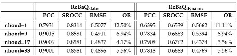
5.2. Model Parameter Selection

The proposed quality index accepts four parameters: 1)nhood, dimensions of the window centered around the current pixel for calculating theds; 2)L, number of multi-scale levels; 3)βs, used in the

calculation ofPD,s,l(x,y)in Equation (6); and 4)βc, used in the calculation ofPD,c,l(x,y)in Equation (8).

(18)

static dynamic

PCC SROCC RMSE OR PCC SROCC RMSE OR

nhood=1 0.7931 0.8314 0.5077 12.50% 0.6395 0.6539 0.5662 11.11% nhood=9 0.9015 0.8581 0.4911 6.94% 0.7834 0.6683 0.5394 6.94% nhood=17 0.9006 0.8581 0.4837 4.17% 0.7908 0.6762 0.4374 5.56% nhood=33 0.9001 0.8581 0.4896 5.56% 0.7818 0.6683 0.4769 5.56%

(b)Simulation results with different number of scalesL

ReBaQstatic ReBaQdynamic

PCC SROCC RMSE OR PCC SROCC RMSE OR

L=1 0.8190 0.8183 0.6667 8.33% 0.5561 0.5520 0.7335 12.50% L=2 0.8597 0.8310 0.5521 5.56% 0.7281 0.6482 0.6050 5.56% L=3 0.9006 0.8592 0.5077 4.17% 0.7908 0.6773 0.5662 5.56% L=4 0.9006 0.8581 0.4915 4.17% 0.7954 0.6797 0.5350 5.56% L=5 0.9006 0.8581 0.4883 5.56% 0.8087 0.6881 0.5191 5.56%

the neighborhood search window size as expected, but the performance of RBQI increased drastically for the ReBaQdynamicdataset fromnhood = 1 tonhood = 17 before starting to drop atnhood = 33.

Thus we chosenhood=17 for all our experiments. Table4(b)gives performance results for different number of scales. As a tradeoff between the computation complexity and prediction accuracy we chose the number of scales to beL=3. The probability summation model parametersβsandβcwere

found such that they maximized the correlation between RBQI and MOS scores on ReBaQ dataset. As in [60], we divided the ReBaQ dataset into two subsets by randomly choosing 80% of the total images for training and 20% for testing. The random training-testing procedure was repeated 100 times and the parameters were averaged over the 100 iterations. Valuesβs =3.5βc=3.5 were found to correlate

well with the subjective test scores.

These parameters remained unchanged for the experiments conducted on the S-ReBaQ dataset to obtain the values in Table2and3.

6. Conclusion

In this paper we addressed the problem of quality evaluation of reconstructed background images. We first proposed two different datasets for benchmarking the performance of existing and future techniques proposed to evaluate the quality of reconstructed background images. Then we proposed the first full-reference Reconstructed Background Quality Index (RBQI) to objectively measure the perceived quality of the reconstructed background images.

(19)

showed that the proposed measure out-performed all the existing statistical and IQA techniques in estimating the perceived quality of reconstructed background images.

The proposed RBQI has multiple applications. It can be used by the algorithm developers to optimize the performance of their techniques, by users to compare different background reconstruction algorithms and to determine which algorithm is best suited for there task. It can also be deployed in challenges (e.g. SBMC [22]) that promote the development of improved background reconstruction algorithms. As future work, the authors will be investigating the development of a no-reference quality index for assessing the perceived quality of reconstructed background images in scenarios where the reference background images are not available. The no-reference metric can also be used as a feedback to the algorithm to adaptively optimize its performance.

Supplementary Materials:The ReBaQ and S-ReBaQ datasets and source code for RBQI will be available for download at the authors’ websitehttps://github.com/ashrotre/RBQIorhttps://ivulab.asu.edu.

Author Contributions: Aditee Shrotre and Lina Karam contributed to the design and development of the proposed method and to the writing of the manuscript. Aditee Shrotre contributed additionally to the software implementation and testing of the proposed method.

Abbreviations

The following abbreviations are used in this manuscript:

RBQI Reconstructed Background Quality Index PSNR Peak Signal to Noise Ratio

AGE Average Gray-level Error EPs Number of Error Pixels pEPs percentage of Error Pixels CEPs number of Clustered Error Pixels pCEPs percentage of Clustered Error Pixels IQA Image Quality Analysis

FR-IQA Full Reference Image Quality Assessment HVS Human Visual System

MS-SSIM Multi-scale Structural SIMilarity index CQM Color image Quality Measures

PETS Performance Evaluation of Tracking and Surveillance SBMNet Scene Background Modeling Net

SSIM Structural SIMilarity index VSNR Visual Signal-to-Noise ratio VIF Visual Information Fidelity

VIFP pixel-based Visual Information Fidelity UQI Universal Quality Index

IFC Image Fidelity Criterion NQM Noise Quality Measure WSNR Weights Signal-to-Noise Ratio FSIM Feature SIMilarity index

FSIMc Feature SIMilarity index with color SR-SIM Spectral Residual SIMilarity index SalSSIM Saliency-based Structural SIMilarity index ReBaQ Reconstructed Background Quality dataset

S-ReBaQ SBMNet based Reconstructed Background Quality dataset SBMC Scene Background Modeling

MOS Mean Opinion Score

PCC Pearson Correlation Coefficient

SROCC Spearman Rank Order Correlation Coefficient RMSE Root Mean Square Error

(20)

and Images, 2011, pp. 297–304.

2. Stauffer, C.; Grimson, W.E.L. Learning patterns of activity using real-time tracking. IEEE Transactions on Pattern Analysis and Machine Intelligence2000,22, 747–757.

3. Li, L.; Huang, W.; Gu, I.Y.H.; Tian, Q. Statistical modeling of complex backgrounds for foreground object detection. IEEE Transactions on Image Processing2004,13, 1459–1472.

4. Fleuret, F.; Berclaz, J.; Lengagne, R.; Fua, P. Multicamera People Tracking with a Probabilistic Occupancy Map. IEEE Transactions on Pattern Analysis and Machine Intelligence2008,30, 267–282.

5. Flores, A.; Belongie, S. Removing pedestrians from google street view images. Proc. IEEE Computer Society Conference on Computer Vision and Pattern Recognition Workshops, 2010, pp. 53–58.

6. Jones, W.D. Microsoft and Google vie for virtual world domination.IEEE Spectrum2006,43, 16–18. 7. Zheng, E.; Chen, Q.; Yang, X.; Liu, Y. Robust 3D modeling from silhouette cues. Proc. IEEE International

Conference on Acoustics, Speech and Signal Processing, 2009, pp. 1265–1268.

8. Maddalena, L.; Petrosino, A. A Self-Organizing Approach to Background Subtraction for Visual Surveillance Applications. IEEE Transactions on Image Processing,2008,17, 1168–1177.

9. Varadarajan, S.; Karam, L.; Florencio, D. Background subtraction using spatio-temporal continuities. Proc. European Workshop on Visual Information Processing, 2010, pp. 144–148.

10. Farin, D.; de With, P.; Effelsberg, W. Robust background estimation for complex video sequences. Proc. IEEE International Conference on Image Processing, 2003, Vol. 1, pp. 145–148.

11. Hsiao, H.H.; Leou, J.J. Background initialization and foreground segmentation for bootstrapping video sequences.EURASIP Journal on Image and Video Processing2013, p. 12.

12. Reddy, V.; Sanderson, C.; Lovell, B. A low-complexity algorithm for static background estimation from cluttered image sequences in surveillance contexts.EURASIP Journal on Image and Video Processing2010, pp. 1:1–1:14.

13. Yao, J.; Odobez, J. Multi-Layer Background Subtraction Based on Color and Texture. Proc. IEEE Conference on Computer Vision and Pattern Recognition„ 2007, pp. 1–8.

14. Colombari, A.; Fusiello, A. Patch-Based Background Initialization in Heavily Cluttered Video. IEEE Transactions on Image Processing2010,19, 926–933.

15. Herley, C. Automatic occlusion removal from minimum number of images. Proc. IEEE International Conference on Image Processing, 2005, Vol. 2, pp. 1046–1049.

16. Agarwala, A.; Dontcheva, M.; Agrawala, M.; Drucker, S.; Colburn, A.; Curless, B.; Salesin, D.; Cohen, M. Interactive Digital Photomontage. ACM Transactions on Graphics2004,23, 294–302.

17. Shrotre, A.; Karam, L. Background recovery from multiple images. Proc. IEEE Digital Signal Processing and Signal Processing Education Meeting, 2013, pp. 135–140.

18. Maddalena, L.; Petrosino, A. Towards Benchmarking Scene Background Initialization. Proc. International Conference on Image Analysis and Processing, 2015, pp. 469–476.

19. Wang, Z.; Simoncelli, E.; Bovik, A. Multiscale structural similarity for image quality assessment. Proc. Asilomar Conference on Signals, Systems and Computers, 2003, Vol. 2, pp. 1398–1402.

20. Yalman, Y.; Ertürk, ˙I. A new color image quality measure based on YUV transformation and PSNR for human vision system. Turkish Journal of Electrical Engineering & Computer Sciences2013,21, 603–612. 21. Bouwmans, T.; Maddalena, L.; Petrosino, A. Scene background initialization: A taxonomy. Pattern

Recognition Letters2017,96, 3–11.

22. Maddalena, L.; Jodoin, P. http://www.icpr2016.org/site/session/scene-background-modeling-sbmc2016/.

23. Toyama, K.; Krumm, J.; Brumitt, B.; Meyers, B. Wallflower: principles and practice of background maintenance. Proc. IEEE International Conference on Computer Vision„ 1999, Vol. 1, pp. 255–261. 24. Li, L.; Huang, W.; Gu, I.H.; Tian, Q. Statistical modeling of complex backgrounds for foreground object

detection. IEEE Transactions on Image Processing,2004,13, 1459–1472.

(21)

26. Sheikh, Y.; Shah, M. Bayesian modeling of dynamic scenes for object detection.IEEE Transactions on Pattern Analysis and Machine Intelligence2005,27, 1778–1792.

27. Jodoin, P.; Maddalena, L.; Petrosino, A.www.SceneBackgroundModeling.net.

28. Shrotre, A.; Karam, L. Visual quality assessment of reconstructed background images. Proc. International Conference on Quality of Multimedia Experience, 2016, pp. 1–6.

29. Wang, Z.; Bovik, A.; Sheikh, H.; Simoncelli, E. Image quality assessment: from error visibility to structural similarity. IEEE Transactions on Image Processing2004,13, 600–612.

30. Chandler, D.; Hemami, S. VSNR: A Wavelet-Based Visual Signal-to-Noise Ratio for Natural Images.IEEE Transactions on Image Processing2007,16, 2284–2298.

31. Sheikh, H.; Bovik, A. Image information and visual quality. IEEE Transactions on Image Processing2006,

15, 430–444.

32. Wang, Z.; Bovik, A. A universal image quality index.IEEE Signal Processing Letters2002,9, 81–84. 33. Sheikh, H.; Bovik, A.; de Veciana, G. An information fidelity criterion for image quality assessment using

natural scene statistics. IEEE Transactions on Image Processing2005,14, 2117–2128.

34. Damera-Venkata, N.; Kite, T.; Geisler, W.; Evans, B.; Bovik, A. Image quality assessment based on a degradation model. IEEE Transactions on Image Processing2000,9, 636–650.

35. Mitsa, T.; Varkur, K. Evaluation of contrast sensitivity functions for the formulation of quality measures incorporated in halftoning algorithms. Proc. IEEE International Conference on Acoustics, Speech, and Signal Processing, 1993, Vol. 5, pp. 301–304.

36. Zhang, L.; Zhang, D.; Mo, X.; Zhang, D. FSIM: A Feature Similarity Index for Image Quality Assessment.

IEEE Transactions on Image Processing2011,20, 2378–2386.

37. Zhang, L.; Li, H. SR-SIM: A fast and high performance IQA index based on spectral residual. Proc. IEEE International Conference on Image Processing, 2012, pp. 1473–1476.

38. Akamine, W.; Farias, M. Incorporating visual attention models into video quality metrics. SPIE Proceedings, 2014, Vol. 9016, pp. 1–9.

39. Laugraud, B.; Piérard, S.; Van Droogenbroeck, M. LaBGen-P: A pixel-level stationary background generation method based on LaBGen. Proc. International Conference on Pattern Recognition, 2016, pp. 107–113.

40. Maddalena, L.; Petrosino, A. Extracting a background image by a multi-modal scene background model. Proc. International Conference on Pattern Recognition, 2016, pp. 143–148.

41. Javed, S.; Jung, S.K.; Mahmood, A.; Bouwmans, T. Motion-Aware Graph Regularized RPCA for background modeling of complex scenes. Proc. International Conference on Pattern Recognition, 2016, pp. 120–125. 42. Liu, W.; Cai, Y.; Zhang, M.; Li, H.; Gu, H. Scene background estimation based on temporal median filter

with Gaussian filtering. Proc. International Conference on Pattern Recognition, 2016, pp. 132–136. 43. Ramirez-Alonso, G.; Ramirez-Quintana, J.A.; Chacon-Murguia, M.I. Temporal weighted learning model for

background estimation with an automatic re-initialization stage and adaptive parameters update.Pattern Recognition Letters2017,96, 34–44.

44. Minematsu, T.; Shimada, A.; Taniguchi, R.I. Background initialization based on bidirectional analysis and consensus voting. Proc. International Conference on Pattern Recognition, 2016, pp. 126–131.

45. Piccardi, M. Background subtraction techniques: A review. Proc. IEEE International Conference on Systems, Man and Cybernetics, 2004, Vol. 4, pp. 3099–3104.

46. Halfaoui, I.; Bouzaraa, F.; Urfalioglu, O. CNN-based initial background estimation. Proc. International Conference on Pattern Recognition, 2016, pp. 101–106.

47. Chacon-Murguia, M.I.; Ramirez-Quintana, J.A.; Ramirez-Alonso, G. Evaluation of the background modeling method Auto-Adaptive Parallel Neural Network Architecture in the SBMnet dataset. Proc. International Conference on Pattern Recognition, 2016, pp. 137–142.

48. Ortego, D.; SanMiguel, J.C.; Martínez, J.M. Rejection based multipath reconstruction for background estimation in SBMnet 2016 dataset. Proc. International Conference on Pattern Recognition, 2016, pp. 114–119.

49. Methodology for the subjective assessment of the quality of television pictures. Technical Report ITU-R BT.500-13, International Telecommunications Union, 2012.

(22)

54. Chou, C.H.; Liu, K.C. Colour image compression based on the measure of just noticeable colour difference.

IET Image Processing2008,2, 304–322.

55. Mahy, M.; Eycken, L.; Oosterlinck, A. Evaluation of uniform color spaces developed after the adoption of CIELAB and CIELUV.Color Research & Application1994,19, 105–121.

56. Watson, A.; Kreslake, L. Measurement of visual impairment scales for digital video. 2001, Vol. 4299, pp. 79–89.

57. Watson, A.B. DCT quantization matrices visually optimized for individual images. 1993, Vol. 1913, pp. 1913 – 15.

58. Hontsch, I.; Karam, L.J. Adaptive image coding with perceptual distortion control.IEEE Transactions on Image Processing2002,11, 213–222.

59. VQEG. Final report from the Video Quality Experts Group on the validation of objective models of video quality assessment2000.