Resource location based on partial random walks in networks with resource dynamics

(1)

Resource Location Based on Partial Random Walks

in Networks with Resource Dynamics

V´ıctor M. L´opez Mill´an

∗

, Vicent Cholvi

†

, Luis L´opez

‡

, and Antonio Fern´andez Anta

§

∗_{Universidad CEU San Pablo, Spain,}_{[email protected]} †_{Universitat Jaume I, Spain,}_{[email protected]} ‡_{Universidad Rey Juan Carlos, Spain,} _{[email protected]} §_{Institute IMDEA Networks, Spain,}_{[email protected]}

I. INTRODUCTION

A random walk in a network is a routing mechanism that

chooses the next node to visit (uniformly) at random among the neighbors of the current node. Random walks have been extensively studied in Mathematics, and have been used in a wide range of applications such as statistic physics, population dynamics, bioinformatics, etc. When applied to communica-tion networks, random walks have had a profound impact in algorithms and complexity theory. Some of the advantages of random walks are their simplicity, their small processing power consumption at the nodes, and the fact that they need only local information, avoiding the bandwidth overhead necessary in other routing mechanisms to communicate with other nodes.

An important application of random walks has been the search of resources held in the nodes of a network, also known

as resource location. Roughly speaking, the problem consists

of finding a node that holds a resource starting at somesource node. Random walks can be used to perform such a search as follows. It is checked first if the source node holds the resource. If it does not, the search hops to a random neighbor, that repeats the process. The search proceeds through the network in this way until a node that holds the resource is found. Due to the random nature of the walk, some nodes may be visited more than once (unnecessarily from the search standpoint), while other nodes may remain unvisited for a long time. The number of hops taken to find the resource is called the search length of that walk. The performance of this direct application of random walks to network search has been widely studied [1], [5], [8], [3], [7].

Das Sarma et al. [2] proposed a distributed algorithm to obtain a random walk of a specified length ` in a number of rounds1 _{proportional to} √_`_{. In the first phase, every node}

in the network prepares a number of short (random) walks

departing from itself. The second phase takes place when a random walk of a given length starting from a given source node is requested. One of the short walks of the source node is randomly chosen to be the first part of the requested random walk. Then, the last node of that short walk is processed. One

1_A_round_{is a unit of discrete time in which every node is allowed to send a}

message to one of its neighbors. According to this definition, a simple random walk of length`would then take`rounds to be computed.

of its short walks is randomly chosen, and it isconnectedto the previous short walk. The process continues until the desired length is reached.

Hieungmany and Shioda [4] propose arandom-walk-based

file search for P2P networks. A search is conducted along the concatenation of hop-limited shortest path trees. To find a file, a node first checks its file list (i.e., an index of files owned by neighbor nodes). If the requested file is found in the list, the node sends the file request message to the file owner. Otherwise, it randomly selects a leaf node of the hop-limited shortest path tree, and the search follows that path, checking the file listof each node in it.

Contributions This paper proposes an application to

re-source location of the technique of concatenating partial walks (PW) to build random walks. Two variations are considered, depending on whether the search mechanism first chooses one of the PWs at random and then checks its associated information for the desired resource, or it first checks the associated resource information of all the PWs of the node, and then randomly chooses among the PWs with a positive result. We will refer to the resulting mechanisms as

choose-first PW-RW andcheck-first PW-RW, respectively.

In this work, we are concerned with the resource location problem in networks with dynamic behavior regarding the resources. In particular, we consider a scenario in which resources are randomly placed in the nodes across the net-work. Furthermore, we also consider that instances of a given resource located at different nodes may appear and disappear over time. In this scenario, all the nodes of the network may launch independent searches for different resources (e.g., files), and we are interested in measuring the average performance of searches between anypair of nodes.

(2)

investigate the influence of the resource dynamics. We found that both search mechanisms provide optimal search lengths that are small, and they do not depend heavily on the resource dynamics or on the network type. Finally, we have also compared the performance of the proposed search mechanisms with respect to random walk searches. For the choose-first PW-RW mechanism we have found a reduction in the average search length with respect to simple random walk ranging from around 57% to88%. For the check-first PW-RW mechanism such a reduction is even bigger, achieving reductions above

90%.

II. MODEL

We consider a randomly built network of N nodes and arbitrary topology, with a known degree distribution. This network is an overlay network built of top of a network with full interconnection (e.g., the Internet). Every node holds a set of resources. We focus on a given resource of interest, of which initially there is a number of instances randomly placed in many distinct network nodes. Our resource location problem is defined as visiting one of the nodes that hold the resource starting by a certain node (thesourcenode). For each search, the source node is uniformly chosen at random among all nodes in the network. Resources have a dynamic behavior, i.e., they may appear and disappear from the network nodes. We fix a starting time T0 and consider a later timeTr. Then,

an instance of the resource present in a node atT0 disappears with probability d, while a node without the resource at T0 has an instance at time Trwith probability a. We will used

as an input parameter to characterize resource dynamics, and setaaccordingly, so that the expected number of resources in the network remains the same.

The search mechanism proposed in this paper, referred to as (choose-first or check-first) PW-RW, exploits the idea of efficiently building random walksfrom partial random walks

available at each node of the network. It comprises two stages:

(1) Partial random walks construction: At time T0, every

node i in the network precomputes a set Wi of w random

walks in an initial stage before any search takes place, with the initial distribution of resource instances in the network. Each of these partial walks (PW) has lengths, starts ati, and finishes at the node reached after s hops. During the computation of each PW in Wi, node iregisters the resources held by the s

first nodes in the PW. The last node of the PW is excluded, being included in the PWs departing from it. The registered information will be used by the searches in stage 2.

(2) The search: During the interval (T0, Tr],2 searches are

performed in the network as follows (for the the choose-first PW model). When a search start at a node A, a PW inWAis chosen uniformly at random. Its associated resource

information collected in stage 1 is then queried for the desired

2_{We will consider the system at time}_T

r, in which, as stated above, the dynamic behavior of resource instances is characterized byd. Therefore, the results obtained will reflect the performance of the search mechanism in a worst case scenario, since searches executed in(T0, Tr)will see a probability that an instance disappears less thand.

resource. If the resource was not found in the PW, the search

jumpsto nodeB, the last node of that PW. The process is then

repeated atB, so the search keeps jumping in this way while the results of the queries are negative. When, at a nodeC, the query returns a positive result, the search traverses that PW looking for the resource, until the resource is found or the PW is fully traversed. If the resource is found, the search stops. Otherwise, it means that the information collected in stage 1 for that PW is no longer valid. The search then considers that the result is negative, and the search process continues from the last node of the PW.

In this work, we are interested in the number ofhopsto find a resource, which is defined as thesearch length, and denoted

Ls. Some of these hops arejumps(over PWs) and other are

steps(traversing PWs). In turn, we distinguish betweentrailing

steps, if they are the ones taken when the resource is found,

andunnecessary steps, if they are taken when the resource is

not found. The search length is a random variable that takes different values when independent searches are performed.

The search length distribution is defined as the probability

distribution of the search length random variable.

At this point, we emphasize the difference between the

search just defined and the total walk that supports it,

con-sisting of the concatenation ofpartial walksas defined above. Searches are shorter in length than their corresponding total walks because of the number of steps saved in jumps over PWs in which we know that the resource is not located, although these saving may be reduced by the unnecessary steps due to outdated information within PWs.

Regarding resource dynamics, we realize that searches are executed based on information collected at timeT0 that may be outdated at timeTr, when the queries are performed. Four

cases arise when the information associated with a PW is queried for the resource. A True Negative or TN (case (a)) occurs when no instance of the resource was present in the PW at T0, and the same holds at Tr. A True Positive or TP

(case (b)) occurs when one or more instances are present in the PW at T0 and one or more instances (not necessarily the same ones) are present atTr. The impact of resource dynamics

on the performance of the search mechanism comes from the

False Negatives (FN) and the False Positives (FP). An FN

(case (c)) occurs when there was no instance in the PW atT0, but at least one instance is present at Tr. An FN makes the

search jump over that PW, missing the new instance(s). An FP (case (d)) occurs when there were one or more instances in that PW atT0but all of them are gone atTr and there are

no new instances at Tr. An FP makes the search traverse a

whole PW fruitlessly, since no instances are currently in that PW. Note that the case when all instances disappear from the PW, but some other instance(s) appears in that PW is included in the TP case.

(3)

be found. Therefore and in order to preserve their accuracy, PWs may need to be “refreshed” after some time intervals. We look more into this issue in the Appendix.

III. ANALYSIS OF THEPW-RW MECHANISM

Expected search length As mentioned, above, we are

interested in the expected search lengthLs. It can be obtained

that

Ls=

1

Ptp

·(Pn+s·Pfp) +T , (1)

where Pn, Ptp, and Pfp are the probabilities of choosing

a negative PW (either a TN or a FN), a TP, and a FP, respectively, withPn+Ptp+Pfp= 1, whileT is the expected

number of trailing steps.

The probabilities in Equation 1 are estimated with the following expressions:

Ptp = w X

i=1

w−i X

j=0

P(i, j)· i

w,

Pfp = w−1

X

i=0

w−i X

j=1

P(i, j)· j

w,

Pn = w−1

X

i=0

w−i−1

X

j=0

P(i, j)·w−(i+j)

w = 1−Ptp−Pfp,

(2) whereP(i, j)is the probability that, in thewPWs of a node, there areiPWs that are TP andj PWs that are FP. This value can be computed as P(i, j) =B(w, ptp, i)·B(w−i, pfp, j),

where B(m, q, n) is the coefficient of the binomial distri-bution, ptp is the probability that a given PW is a TP, and pfp is the probability that a given PW at any node is an FP,

conditioned on the fact that it is not a TP. Therefore, in order to evaluate the estimation of the expected search length given by Equation 1, we need to obtain the values ofptp,pfpandT.

The computation of the former two probabilities can be found in the Appendix.

To derive an expression for T we rely on T(r), the expec-tation of that variable conditioned on there being rinstances of the resource in the PW. Then,

T = 1

1−Ppw(0)

·

min{s,R} X

r=1

T(r)·Ppw(r). (3)

The first factor is due to the fact thatT is in fact conditioned on there being at least one instance of the resource in the PW. Now we provide an expression forT(r)as the expectation of the position of the first resource in the PW (conditioned on there being rinstances of the resource in the PW) as

T(r) =

s−r X

i=0



i·



 i−1

Y

j=0

1− r

s−j



·

_r

s−i



. (4)

Each factor in the product of Equation 4 is the probability that there is no instance in thejthposition of the PW, conditioned

on that there is no instance in the previous position. The

final factor outside the product is the probability that there is an instance in theith position conditioned on there are no

instances in the previous positions.

Analysis of check-first PW-RW We analyze now a

vari-ation of the choose first mechanism presented. Suppose the search is currently in a node and it needs to pick one of the PWs in that node to decide whether to traverse it or to jump over it. With the new check-first mechanism, it firstchecksthe associated resource information of all the PWs of the node, and then randomly chooses among the PWs with a positive result, if any (otherwise, it chooses among all PWs of the node, as the original version). Thischeck-first PW-RW mechanism improves the performance of the original (choose-first) PW-RW, since the probability of choosing a PW with the resource increases, with no extra storage space cost. A minor additional difference between the algorithms is that in the check-first version, the resource information is registered from the first

node (the node next to the current node) to the last node in the PW. This change slightly improves the performance of the new version, since the probability of choosing a PW with the resource increases also in the cases where the resource is held by the last node of the PW.

Most of the analysis provided above for the choose-first PW-RW mechanism is still valid for check-first PW-RW. We present here the equations that need to be modified to reflect the new behavior. That is the case of Equations 2 for the probabilities of choosing a PW with a TP, FP and negative result, respectively. Their counterparts follow. Remember that

i andj represent the number of PWs of the node that return a TP result and an FP result, respectively:

Ptp = w X

i=1

w−i X

j=0

P(i, j)· i

i+j,

Pfp = w−1

X

i=0

w−i X

j=1

P(i, j)· j

i+j,

Pn = P(0,0) = 1−Ptp−Pfp, (5)

The expression for the expectation of the number of trailing steps taken when traversing the last PW until the resource is found (Equation 3) is still valid. It usesT(r), the expectation of the position of the first resource in the PW, conditioned on there being r instances of the resource in the PW. Its expression (Equation 4) needs to be modified, since the range of nodes whose resources are associated with the PW has changed from[0, s−1]to[1, s]. The indexes limits and their use in the expression have been updated as necessary in the new expression, which completes the analysis of the check-first PW-RW mechanism:

T(r) =

s−r+1

X

i=1



i·



 i−1

Y

j=1

1− r

s−j+ 1



·

r s−i+ 1



.

IV. PERFORMANCEEVALUATION

(4)

0 20 40 60 80 100 120 140

0 50 100 150 200 250 300 350 400

expected search length (hops)

partial walks size (hops) PW-RW1 (choose first) regular network

d=0.700 (simul) (model) d=0.500 (simul) (model) d=0.300 (simul) (model) d=0.100 (simul) (model) d=0.000 (simul) (model)

(a) Regular network

0 20 40 60 80 100 120 140

0 50 100 150 200 250 300 350 400

partial walks size (hops) PW-RW1 (choose first) ER network

(b) ER network

0 20 40 60 80 100 120 140

0 50 100 150 200 250 300 350 400

partial walks size (hops) PW-RW1 (choose first)

scalefree network

(c) Scale-free network

Fig. 1. Choose-first PW-RW. Expected search length (Ls) vs. PW length (s) ford= 0.0,0.1,0.3,0.5,0.7withw= 5.

simulations. Three types of networks have been chosen for the experiments: regular networks (constant node degree), Erd˝os-R´enyi (ER) networks and scale-free networks (with power law on the node degree). A network of each type and sizeN = 104 has been randomly built with the method proposed by Newman et al. [6] for networks with arbitrary degree distribution, setting their average node degree to k = 10. For each experiment,

106_{searches have been performed. In every search, the source} node has been chosen uniformly at random, and every node in the network has been assigned an instance of the resource with probability pres= 10−2 atT0.

Expected search lengthFigure 1 shows the expected search

length in the three networks, for several values of d. The number of PWs per node is set to w = 5, although the performance of the PW-RW mechanism is almost independent from this parameter, since only one PW is used to locate the resource. (On the contrary, this parameter plays a central role in the check-first PW-RW.) Model predictions (Section II) are plotted with lines and simulation results are shown as points. It can be seen that the model provides an accurate approximation of the real data, with larger error for higher values of dand

s. Among the network types, the regular network shows the smallest errors, followed by the ER network and the scale-free network. These discrepancies are accounted for by the greater dispersion of node degree in the ER, and especially, in the scale-free networks. Predictions ofLs are slightly lower than

experimental data, rendering an optimistic model in general, with a very good fit for interesting values of sand values of

d not large. All curves show a minimum point, which marks the optimal PW length (sopt) and the corresponding optimal

expected search length (Lopt). Interestingly, the values ofsopt

are small and do not depend heavily on dor on the network type. According to the analytic data, sopt ranges between 13

and 15 for all curves shown and for the three network types. Values ofLoptare also very similar. For example, ford= 0.3, Lopt= 21.95(regular), 21.83 (ER), and 21.32 (scale-free).

We have compared the performance of the proposed search mechanism for Lopt with searches based on simple random

walks. Table I shows the relative reductions (%) for several values ofdfor the network types we have considered. We can see that the reduction in the average search length that

choose-choose-first PW-RW check-first PW-RW

d Regular ER Scale-free Regular ER Scale-free 0.0 87.73 87.87 88.26 94.02 94.11 94.29 0.1 85.76 85.87 86.36 93.09 93.20 93.43 0.3 80.24 80.57 81.22 90.59 90.74 91.04 0.5 71.82 72.02 72.93 86.27 86.49 86.91 0.7 55.68 55.95 57.25 77.08 77.43 78.12

TABLE I

REDUCTION(IN%)OF THE EXPECTED SEARCH LENGTHS OF

CHOOSE-FIRSTPW-RWAND CHECK-FIRSTPW-RW (w= 5)RELATIVE

TO RANDOM WALK SEARCHES FOR SEVERALd.

first PW-RW achieves with respect to simple random walk is lower for higherd, ranging from around 87% in the case when

d= 0to 55% whend= 0.7. Furthermore, we also see that the achieved reductions are independent of the network type, with small differences.

Search length distribution The use of partial walks also

affects the shape of the probabilistic distribution of search lengths. Figure 2a shows the distributions for simple random walks (RW) and for choose-first PW-RW, fors= 10and for several values of d, obtained from the experiments with the regular network. Instead of the slowly decaying distribution of random walks, the proposed mechanism exhibits search length distributions that show a maximum frequency for a small search length and then decay much faster than the random walk distribution. We also note that the search length for the maximum frequency (9 in this case) is independent from the dynamic behavior of resources (d). The search length distributions of PW-RW have therefore lower standard devia-tion (and also lower coefficient of variadevia-tion) than the random walk searches. Regarding the ER and the scale-free networks (omitted), their search length distributions have similar shape, mean and standard deviation values.

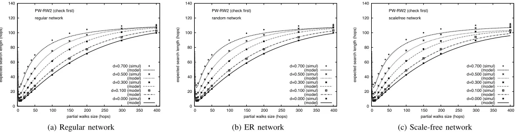
Check-First PW-RWWe look now at the check-first

PW-RW mechanism. Figure 3 shows the expected search length in the three networks for several values ofd, and forw= 5. The shape of the curves is the same as that for the choose-first mechanism (Figure 1), with a substantial decrease in the optimal search length (Lopt). For example, ford= 0.3,Lopt

(5)

0 10000 20000 30000 40000 50000 60000

0 20 40 60 80 100 120

absolute frequency

search length (hops) regular network

PWRW d=0.0 PWRW d=0.1 PWRW d=0.3 PWRW d=0.5 PWRW d=0.7 RW

(a)

0 20 40 60 80 100

0 10 20 30 40 50 60

partial walks size (hops) PW-RW2 (check first) regular network d=0.3

choose-first PW-RW (simul) (model) check-first PW-RW, w=2 (simul) (model) check-first PW-RW, w=5 (simul) (model) check-first PW-RW, w=10(simul) (model)

(b)

Fig. 2. (a) Search length distributions for searches based on random walks and on choose-first PW-RW, for a regular network with s = 10and d= 0,0.1,0.3,0.5and0.7. (b) Expected search length (Ls) vs. PW length (s) for check-first PW-RW withw= 2,5,10, and choose-first PW-RW in a regular network withd= 0.3.

0 20 40 60 80 100 120 140

0 50 100 150 200 250 300 350 400

partial walks size (hops) PW-RW2 (check first)

regular network

d=0.700 (simul) (model) d=0.500 (simul) (model) d=0.300 (simul) (model) d=0.100 (model) (model) d=0.000 (simul) (model)

(a) Regular network

0 20 40 60 80 100 120 140

0 50 100 150 200 250 300 350 400

random network

(b) ER network

0 20 40 60 80 100 120 140

0 50 100 150 200 250 300 350 400

scalefree network

(c) Scale-free network

Fig. 3. Check-first PW-RW. Expected search length (Ls) vs. PW length (s) ford= 0.0,0.1,0.3,0.5,0.7withw= 5.

length also diminishes, from about 14 to 6 in that case. The expected search length decrease is due to the fact that the new mechanism checks all the PWs in the node for the resource and then chooses one only among those with positive result, increasing the probability of choosing a PW that currently holds the resource. Following this reasoning, the more PWs in the node, the higher this probability. It is therefore interesting to explore the dependency of Landsoptwithw.

Figure 2b shows the expected search length of the check-first PW-RW mechanism, forw= 2,5and10in a regular net-work with d= 0.3. To make the comparison of performance between both mechanisms easier, a curve corresponding to choose-first PW-RW has been added to the graph. For higher

s, the curves for the several w converge. As expected, it is observed that higherw yields lowerLopt, with a value about

8 forw= 10. Another interesting observation is thatsoptalso

diminishes for higherw, falling to 4 in this case. These values mean a reduction of about 92% in the expected search length of simple random walks, with 10 precomputed PWs of just 4 nodes. Higher reductions can be achieved, at the expense of increasing the cost of the computation of the PWs. Results for the ER and scale-free networks are similar. Table I is provided as a reference, presenting the reductions achieved by check-first PW-RW forw= 5with respect to random walk searches in a regular, ER and scale-free networks for severald. We see

that reductions range between 94% and 77%, while those of choose-first PW-RW range between 88% and 55%.

REFERENCES

[1] L. A. Adamic, R. M. Lukose, A. R. Puniyani, and B. A. Huberman. Search in power-law networks. Physical Review E, 64(046135), 2001. [2] A. Das Sarma, D. Nanongkai, G. Pandurangan, and P. Tetali. Efficient

distributed random walks with applications. In Proceeding of the 29th ACM SIGACT-SIGOPS symposium on Principles of distributed comput-ing, PODC ’10, pages 201–210, New York, NY, USA, 2010. ACM. [3] C. Gkantsidis, M. Mihail, and A. Saberi. Random-walks in peer-to-peer

networks: algorithms and evaluation. Performance Evaluation, 63:241– 263, 2006.

[4] P. Hieungmany and S. Shioda. Characteristics of random walk search on embedded tree structure for unstructured p2ps. Parallel and Distributed

Systems, International Conference on, 0:782–787, 2010.

[5] Q. Lv, P. Cao, E. Cohen, K. Li, and S. Shenker. Search and replication in unstructured peer-to-peer networks. InICS ’02: Proceedings of the 16th

international conference on Supercomputing, pages 84–95, New York,

NY, USA, 2002. ACM.

[6] M. E. J. Newman, S. H. Strogatz, and D. J. Watts. Random graphs with arbitrary degree distributions and their applications. Physical Review E, 64(026118), 2001.

[7] L. Rodero-Merino, A. Fern´andez Anta, L. L´opez, and V. Cholvi. Per-formance of random walks in one-hop replication networks. Computer

Networks, 54(5):781–796, 2010.

[8] S.-J. Yang. Exploring complex networks by walking on them. Physical

(6)

APPENDIX

A. Cost of Precomputing PWs

Let’s consider the interval (T0, Tr], chosen so that the

probability d at T0 has some acceptable value.3 Searches performed in this interval use the PWs precomputed atT0, and thus the cost of this computation must be added to the cost of the searches themselves. We measure this cost as the number of messages Cp that need to be sent to compute all the PWs

in the network. This quantity has been chosen to be consistent with our measure of the performance of the searches. Indeed, each hop taken by a search can be alternatively considered

as a message sent. In addition,Cp is independent from other

factors like the processing power of nodes, the bandwidth of links and the load of the network.

The cost of precomputing a set of PWs atT0 can be simply obtained as Cp =N w(s+ 1), since each of the N nodes in

the network computeswpartial walks, sendingsmessages to build each of them plus one extra message to get back to its source node.

Let’s suppose that each node starts on the averagebsearches in(T0, Tr]. We defineCs to be the total number of messages

needed to complete those searches. If the expected number of messages of a search is Ls+ 1(counting the message to get

back to the source node), we have thatCs=N b(Ls+1). Now,

defining Ct as the average total cost per search in (T0, Tr],

we can write:

Ct=

Cs+Cp

N b = (Ls+ 1) +

w

b(s+ 1). (6)

The second term in Equation 6 is the contribution to the cost of the precomputation of the PWs inT0. This contribution will remain small provided that the number of searches per node in the interval is large enough.

B. Computation of ptp and pfp

The variable ptp has been defined as the probability that a

given PW at any node returns a TP result. This probability can be easily estimated if we condition it on the fact that the PW (of lengths) had exactlyrinstances of the resource atT0. Defining Ppw(r)as the probability that a PW hasrinstances

of the resource, and recalling thatR is the expectation of the number of instances of the resource in the network, we can write:

ptp=

min{s,R} X

r=1

Ppw(r)·(1−dr) +dr· 1−(1−a)s−r,

(7) where the brackets contain the probability that not all the r

instances present atT0 have disappeared (with probabilityd) at Tr or, if they did disappear, at least one instance appeared

3_{The interval for which the dynamic behaviour of resources yields a given}

value ofddepends on the stochastic processes that governs the births and deaths of resource instances in the nodes of the network. The determination of that interval is out of the scope of this work.

(with probability a) in some of thes−r remaining nodes in that interval.

An estimation forPpw(r)can be obtained using the random

properties of a random walk in networks built randomly. In particular, we consider that the next hop of a random RW can take it to any of the endpoints in the network (except the endpoints of the current node since we do not allow self-loops). Then we estimate Ppw(r)as B(s, prw, r), whereprw

is the probability that the RW visits a node with an instance of the resource in the next hop. In turn, we estimate this probability as:

prw= R·k

S−krw

·krw−1

krw

. (8)

The first fraction in Equation 8 is the ratio of positive endpoints (the ones connected to the R nodes that have an instance of the resource) and all endpoints in the network (S = P

kk nk) except those of the current node. We use

the average degree of the network (k = P

kk nk/N) as an

estimation of the degree of a node that holds the resource (which is assigned or not with uniform probabilitypresacross

the network). Similarly, we use the expectation of the degree of a node visited by a random walk as an estimation of the degree of the current node:

krw= X

k

k· k·nk

S =

1

S · X

k

k2·nk. (9)

The second fraction in Equation 8 corrects the previous ratio taking into account that, when at a node of a given degree, the probability of not going backwards (and therefore having the chance to find the resource) is the probability of selecting any of its endpoints but the one that connects it with the node just visited by the walk. With this, the estimation ofPpw(r)

is:

Ppw(r) =

s r

·(prw)r·(1−prw)s−r. (10)

We have defined pfp as the probability that a given PW at

any node returns a FP result, conditioned on the fact that it does not return a TP. This conditioning comes from the second binomial coefficient in this equation, which we restrict to the

w−iPWs which we know that do not return a TP, since the ones that do are accounted for in the first binomial coefficient. In other words, the second binomial coefficient includes the PWs that return a TN, a FN or a FP result, and pfp is the

probability that it returns a FP conditioned on that. We can then easily write an estimation ofpfp as:

pfp=

1

1−ptp

(1−Ppw(0)−ptp), (11)

where we are substracting Ppw(0) (the probability of cases