*Corresponding author: [email protected]
2017 UTHM Publisher. All right reserved. 25
penerbit.uthm.edu.my/ojs/index.php/jst
The Performance of K-Means and
K-Modes Clustering to Identify Cluster in Numerical Data
Nur Atiqah Hamzah*, Sie Long Kek and Sabariah Saharan
Department of Mathematics and Statistics, Faculty of Applied Sciences and Technology, Universiti Tun Hussein Onn Malaysia, 86400 Parit Raja, Batu Pahat, Johor, Malaysia.
Received 30 September 2017; accepted 4 December 2017; available online 12 December 2017
1. Introduction
Mean and mode are two well-known measure of central tendency which are used as statistical measure to identify single value as representative of entire distribution. Mean is commonly used and the benefit of using mean is that this measure uses every value in the data to obtain its value. It was claimed that mean is the best measure of central tendency that resist fluctuation between different samples. However, it is very sensitive to extreme values and outliers; not suitable with data with skewed distribution. Meanwhile, mode is the most frequent in dataset. The mode is not affected by extreme values and can be used for both qualitative and quantitative data.
There are clustering techniques which are introduced based on central tendency deviation principle [1]. Clustering analysis is one of the most frequently used data mining techniques [2]. Clustering is an unsupervised learning task with purpose to make natural groupings based on similarity [3]. Clustering process will divide the data sets that have
similarities into same cluster group whereas objects that belong to the other clusters are as dissimilar as possible. Cluster analysis is used to separate data elements into groups by maximizing the homogeneity within elements of clusters and heterogenity between clusters [4]. Clustering is also known as unsupervised learning algorithm because the actual number of clusters is unknown [5].
In this study, two clustering techniques are used, which are K-means clustering and
K-modes clustering. K-means clustering was proposed by MacQueen (1967) and it is still been used by many researchers for many years due to its simplicity computations. K-means clustering is known as hard clustering since each data point belongs to one cluster only [6].
K-means algorithm is based on the center of the associated cluster [7]. By using K-means clustering, the data is put into homogenous cluster which means that the groups have identical characteristics; in terms of intra-cluster similarity [8].
On the other hand, K-modes clustering uses similar concept of K-means but removes the limitation of numeric data. K-modes clustering is used for categorical data which
Abstract: Cluster analysis is a formal study of methods and algorithms for natural grouping of objects according to the perceived intrinsic characteristics and the measure similarities in each group of the objects. The pattern of each cluster and the relationship for each cluster are identified, then they are related to the frequency of occurrence in the data set. Meanwhile, the mean and the mode are known as the measures of central tendency in a distribution. In clustering, the mean and the mode are applied as a technique to discover the existing of the cluster in the data set. Therefore, this study aims to compare the performance of K-means and K-modes clustering techniques in finding the group of cluster that exists in the numerical data. The difference between these methods is that the K-modes method is usually applied to categorical data, while
K-means method is applied to numerical data. However, both methods would be used to cluster the numerical data in this study. Moreover, performance of these two clustering methods are demonstrated using the output from R software. The results obtained are compared such that the method giving the best output could be determined. In conclusion, the efficiency of the methods is highly presented.
26
adjusting K-means method by substitute Euclidean distance metric with simple matching dissimilarity measure. This technique uses modes to represent cluster centers and updating modes with the most frequent categorical values in each iteration of clustering process. The advantages of
K-modes is, it is scalable to very large data sets. However, random initial modes may lead to non-repetitive clustering structures formation [9]. In 2016, a study had implemented K-modes clustering on Iris dataset by transforming the data into binary data [10]. However, in this study, no modifications are made on data.
This study has three main objectives:
i. To apply K-means and K-modes on numerical data.
ii. To differentiate the clustering output using different methods.
iii. To measure the efficiency of mean and mode as clustering methods.
Based on clustering output, the performance of these two techniques are differentiated and this study aims to show if these clustering methods obey central tendency measure.
2. Methodology
This study applies two clustering methods which are K-means and K-modes clustering methods in order to identify the differences of both methods. The clustering method minimizes the following function
where
The selection of k clustermust be smaller than the number of object in the data set [11]. Usually, the number of k is started with the small value. In this study, k=3 is chosen because it gave good clustering result for both data when K-means clustering is applied. Meanwhile, the same value of k is used in
K-modes clustering. It is because this study wants to make comparison on the clustering result when the value of k is fixed. The methodology of each methods are further discussed in Sections 2.1 and 2.2. Both
clustering methods are performed by using the R Software.
2.1 K-means Clustering
In K-means clustering process, number of clusters is set to k=3. The centroids are selected randomly from the dataset for each cluster. The distance of data points to the centroid is calculated using selected distance measure. Each point is placed in the group based on the shortest distance to the centroid. The centroid value is then updated by finding the mean of the elements in the groups. The formal K-means clustering algorithm is given as follows:
Step 1 Choose a value k.
Step 2 Select points as initial centroids. Step 3 Calculate the distance of points to
centroids.
Step 4 Assign points to group based on distance computed.
Step 5 Update the centroid by finding the means.
Step 6 Repeat Steps 3, 4 and 5.
Step 7 Stop the process when there is no more changes in each group.
2.2 K-modes Clustering
The process of K-modes clustering does not have so much different than K-means clustering. By setting the value of k cluster, number of initial centres is selected which correspond to the value of k. Then, distances are calculated. The mode values are updated and the process are continued until there is no changes in the clusters.
In this study, the number of cluster for
K-modes clustering is set to k=3; which is same with K-means clustering. However, the distance is calculated using simple-matching distance. The steps to perform the K-modes clustering are as below:
Step 1 Choose a value of k.
Step 2 Select initial centres (modes). Step 3 Calculate the distances between
objects to the cluster modes.
Step 4 Update the modes value and repeat the step to calculate the distances.
, , ,
1 1 1
( , ) ( , )
k n m
i l i j l j l i j
F U Z u d x z
,
1 2
is an ( ) partition matrix,
{ , ,..., } is a set of mean or mode vectors , distance
i j
k
U u n k
Z Z Z Z d
27
Step 5 Stop the process when no changes on cluster membership.
3. Results and Discussion
This study uses two data to make comparison of output using four types of distance measure. The first data is the Iris data from the UCI Machine Learning website which has four numeric, predictive attributes and class. The Iris data has been used widely for research purposes. Meanwhile, the second data used is the Malaysia household incomes data that have not been used for clustering purposes. The data were given by Micro Data UTHM which handled is in the Department of Mathematics and Statistics of Faculty of Science, Technology and Human Development. The household data have four numeric attributes which are employment incomes, self-employment incomes, property income and transfers received.
Table 1 shows two types of dataset information that have been used in this study. Both data are multivariate dataset. The Iris dataset has 150 instances, four real attributes and no missing value included. While, the household income dataset, which is also multivariate data, has 500 instances, four real attributes and no missing value in the dataset.
Table 1 Dataset information.
Name of dataset
Iris Income
Dataset
Characteristics Multivariate Multivariate Number of
Instances 150 500
Number of
Attributes 4 4
Missing Value No No
Attribute
Characteristics Real Real
Area Life Economy
3.1 Clustering on Iris Dataset
Both K-means and K-modes clustering methods are applied on the Iris dataset. The number of clusters k=3 was set to both clustering processes. However, only two attributes were selected for clustering process which are petal length and petal width.
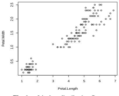
Fig. 1 shows distribution of the Iris data of petal length against petal width. Based on the figure, there are two main groups. However, the value of k was set to 3 because the types of the Iris data are known which are setosa, versicolor and virginica.
Fig. 1 Iris data distribution figure.
3.1.1 K-means Clustering on Iris Dataset
K-means clustering was performed on the Iris dataset. Fig. 2 shows the command used to call the Iris dataset from the library of the R software. The head(iris)command shows variables of the Iris dataset and the first six data values.
Fig. 2 Command to import dataset from library
Fig. 3 shows the output of clustering process using the R software. Three clusters have different sizes which are 48, 52 and 50 respectively. Each cluster has its own cluster means value for each variable. The value of within cluster sum of squares by cluster are 16.29167, 13.05769 and 2.02200, respectively.
1 2 3 4 5 6 7
0
.5
1
.0
1
.5
2
.0
2
.5
Petal.Length
P
e
ta
l.W
id
28
Fig. 3 Cluster outputs for Iris dataset
Fig. 4 shows the commands and outputs to identify clusters centers in table form, number of iterations, total sum of squares, within cluster sum of squares and between cluster sum of squares. From the output, total sum of squares for the Iris K-means clustering is 550.8953, and between cluster sum of squares are 519.524. The smallest within cluster sum of squares is 2.02200 by the third cluster; followed by the second cluster (13.05769) and the first cluster (16.29167).
Fig. 4 Output of K-means clustering
In Fig. 5, a table is formed. The table shows the number of each types of the Iris species in every clusters. All setosa types are put into the third cluster. There are two instances in the first cluster and 48 instances in the second cluster for versicolor. Meanwhile, 46 instances of virginica are put into the first cluster and the remaining 4 instances are put into the second cluster. This shows that every species has strong similarities on petal length and petal widths. The high percentage of between sum of squares over total sum of squares proved that the K-means clustering gave good clustering outputs on the Iris dataset.
Fig. 5 Output shows table of Iris species in each clusters formed
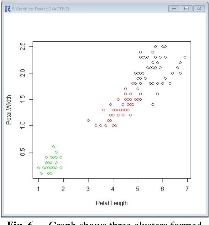
Fig. 6 shows the clusters formed using
K-means clustering. The different colours on the graph indicate three clusters formed.
Fig. 6 Graph shows three clusters formed on Iris dataset
3.1.2 K-modes Clustering on Iris Dataset
K-modes clustering was applied to the Iris dataset to formed three clusters. The variables used were remained the same. Fig. 7 shows the command used to perform the
29
Fig. 7 Command and outputs of K-modes clustering on Iris dataset
Fig. 8 shows cluster size and the modes value of each cluster. The first cluster has the biggest number of members which are 128 instances. The instances in the second cluster only 15 and the third cluster only 7.
Fig. 8 Cluster size and cluster modes value
Fig. 9 shows number of every species in each cluster. All setosa species are put into first cluster. The versicolor species are put into all the three clusters; 31 instances in the first cluster, 12 instances in the second cluster and 7 instances in the third cluster. Meanwhile, the virginica belongs to two clusters; 47 instances in the first cluster and 3 instances in the second clusters.
Fig. 9 Table of Iris species in each cluster
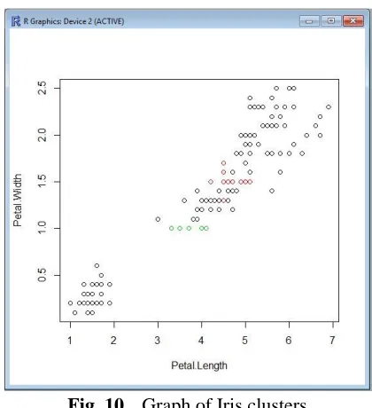
Fig. 10 shows the graph of the Iris dataset. The different colour of the data indicates different clusters. As shown in the
graph, most of the data belongs to the first cluster.
Fig. 10 Graph of Iris clusters
3.2 Clustering on Income Dataset
Clustering methods were applied on income dataset with n=500. Two variables were selected for this clustering process which are employment income and self-employment income. The result of the clustering processes are further discussed in Sections 3.2.1 and 3.2.2.
3.2.1 K-means Clustering on Income Dataset
Although the number of classes of income is unknown, but the value of cluster k is set to 3. It is because this study wants to compare the clustering outputs with the Iris dataset clustering outputs.
30
Fig. 11 Outputs of K-means clustering.
Table 2 shows the value of each cluster center for both variables. The members of each cluster have the smallest sum of squares towards their respective centers value.
Table 2 Cluster center value
Employment income
Self-employment income
1 5811.6837 8964.0244
2 13789.5882 17249.0833
3 71117.2353 93508.6489
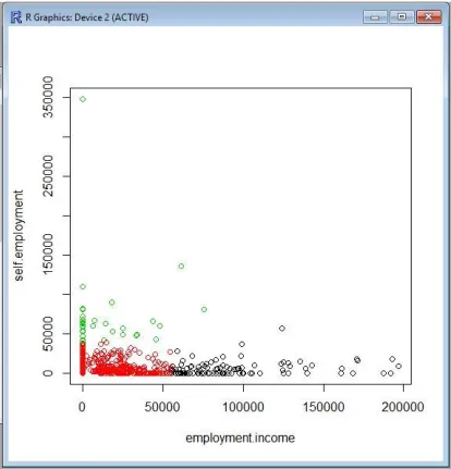
Fig. 12 shows the income graph with three different clusters. From the graph, most of the data are grouped with red colour. The green colour shows the least number of the third cluster members.
Fig. 12 Graph of data distribution with the respective clusters
3.2.2 K-modes Clustering on Income
Dataset
The income dataset are used to carry out
K-modes clustering. The value of cluster k=3 was used and the results from the clustering process were obtained. Figure 13 shows the
K-modes clustering output on incomes data. The cluster sizes are 498, 1, and 1, which shows that from 500 data, 99.6% belongs to only one cluster.
Fig. 13 K-modes outputs on income dataset
Table 3 shows the simple-matching distance of each cluster. The total distance of the first cluster is 764. Meanwhile, the second and the third clusters have zero simple-matching distance. This is due to only one member in the second and the third clusters.
Table 3 Cluster simple-matching distance
Cluster 1 2 3
Simple-matching distance
764 0 0
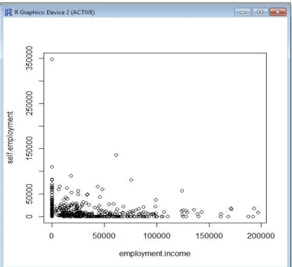
Fig. 13 shows the graph of income data after the clustering process. Due to imbalance number of data in each cluster, the clusters cannot be differentiate clearly by the graph. This shows that most of the data belongs to only one cluster.
Variable
le Cluste r
31
Fig. 13 Graph of income data after K-modes clustering
3.3 Discussion
In this study, two numerical datasets are used to perform K-means and K-modes clustering methods. Both methods used different approach to find distance of the clusters. K-means clustering used sum of squares error value while K-modes used simple-matching coefficient to identify the distance. Using the Iris dataset, K-means clustering gave a better output than K-modes clustering. It is because the clusters formed are clear and the percentage of between cluster sum of square over total sum of square is also high. Besides, the clusters formed by using
K-modes cannot differentiate the Iris species as well.
Meanwhile, using income dataset,
K-means clustering is well performed with 62.4% which is percentage of between cluster sum of square over total sum of square. It indicates that difference of each cluster to the other cluster is maximized. It shows that the
K-means clustering on income dataset gave a better output as K-modes clustering put 99.6% into the same cluster.
4. Conclusion
It was known that mean and mode are two types of measure of central tendency. Thus, this study wanted to investigate how both mean and mode work on clustering process. As this study used two numerical data, the results were compared and discussed. It shows that
K-means performed better clustering process
than K-modes. The distance formulae applied on K-means and K-modes also contribute on the difference performance of clustering process. The sum of square and mean value calculation in K-means clustering gave better output than K-modes clustering which used simple-matching distance and mode value as their centroid. Although in measuring central tendency the mode can be used both on numerical and binary data, however, it was found that K-modes clustering cannot perform well on numerical data. Thus, it is suggested that the data should be transformed into binary data if the K-modes clustering is used.
In conclusion, K-means clustering gives a better output than K-modes clustering on numerical datasets.
Acknowledgements
Authors would like to express greatest gratitude to Research, Innovation, Commercialization, Consultancy Office UTHM (ORICC) for giving the chance to carry out the research by using Geran Penyelidikan Pascasiswazah (GPPS). Authors were extremely thankful to reviewers for their beautiful remarks.
References
[1] Ah-Pine, J. (2009). “Cluster Analysis Based on The Central Tendency Deviation” on Advanced Data Mining and Applications, pp5-18.
[2] Solarte, J. (2002). “A Proposed Data Mining Methodology and Its Application To Its Industrial Engineering”.Unpublished Master’s Degree dissertation, University of Tennessee.
[3] Kruse, R., Doring, C., and Lesot, M.J. (2007). Advances in Fuzzy Clustering and Its Application. John Wiley & Sons, Ltd.
[4] Hair,J.F.jr.,Anderson,R.E.,
Tantham,R.L., Black,W.C. (1998). Multivariate Data Analysis. Prentice Hall.
32
[6] Bora,D.J., and Gupta, A.K. (2014). “A Comparative Study Between Fuzzy Clustering Algorithm and Hard Clustering Algorithm” on International Journal of Computer Trends and Technology (IJCTT), Vol.10 pp108-113. [7] Faber,V. (1994). Clustering and the continuous K-means algorithm. Los Alamos Science, pp138-144.
[8] Anderberg and Michael, R (1973). Cluster Analysis for Applications. New York: Academic Press.
[9] Khan, S., and Kant, S. (2007). “Computation of Initial Modes for K-modes Clustering Algorithm Using Evidence Accumulation” on IJCAI International Joint Conference on Artificial Intelligence, pp2784-2789. [10] Prakash, A., Kalera, S., Tomar, S., Rai,
A., Reddy, P., and Babu, R. (2016). “Review on K-mode Clustering” on International Journal of Engineering and Computer Science, Vol. 5.No 11 pp19054-19062.